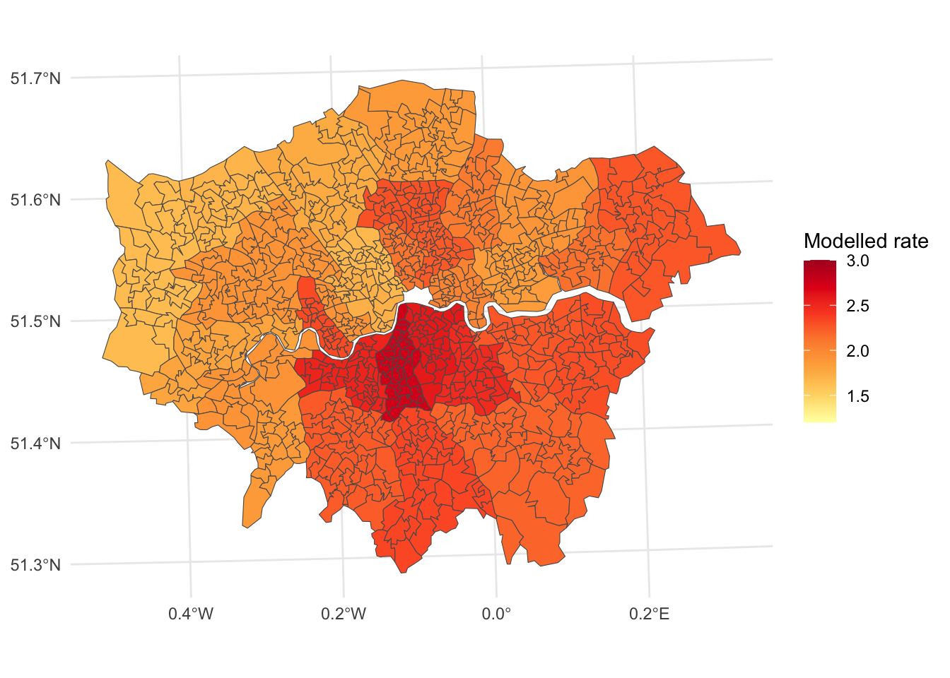
Geographically Weighted Regression, which we looked at in the previous session, treats geographic space as a continuous spatial variable in the sense that regression relationships can vary from one location to another across a geographic study region. That continuous view of space is clear if we fit a simple ‘null model’ of the COVID-19 rates in London in the week before Christmas 2021 and map the results. It is a null model because it includes no predictor variables other than the local estimate of the intercept (i.e. the local mean rate of COVID-19). What is clear is how that local estimate is allowed to vary across geographic space.
(Download and extract the data for London and fit the GWR model)
Multilevel models, by contrast, have more of a discrete view of space because observations at some base level are treated as members of a group at a second, more aggregate level. In a geographic context, the base level could be neighbourhoods and the groups could be the local authorities to which the neighbourhoods belong. This more discrete view of space becomes clear if we fit a very simple (too simple, really) null model of the COVID-19 rates in London, using the local authority estimates from this multilevel model as the nearest equivalent to the local means of the GWR model.
If we compare the map above with that produced from the GWR estimates then we find that there are commonalities in the two maps but the multilevel model clearly has the more bounded view of geographic space.
Multilevel models
The package that we are using to fit the models here is lme4. The formula rate ~ (1|LtlaName) means that we are modelling the COVID-19 rate against a random intercept that varies by local authority (by local authority name, LtlaName). It is not the only way of fitting multilevel models in R (an alternative, for example, is brms) but it is sufficient for the purposes of this exercise.
The more discrete and bounded view of geographic space that the multilevel model (in its simplest form, at least) employs seems quite restricting – in this case study it is suggesting that the causes of COVID-19 are somehow related to ‘things’ that happen or have consequences at a local authority scale. The implication is that the boundaries of local authorities are relevant to the geographical causes and rates of COVID-19. This is not an assumption that GWR makes so why use multilevel models instead?
One answer is that a multilevel model is often faster to fit. Consider the following example, which extends the study region to London and the South East.
Admittedly, neither took very long to fit, with the GWR taking 0.05 minutes and the multilevel model (MLM) taking 0.01 seconds on my laptop. However, these differences become more noticeable with more complex models or larger study regions. The multilevel model is estimating far fewer model parameters than the GWR. This is because the GWR is really lots of models that are fitted separately (one for each location) and then compared, whereas the multilevel model is one model but one which allows for variance at the geographic level(s) of the model, so better local authorities, for example. Put another way, the GWR is a series of local models that are compared, whereas the multilevel model is a global model that allows for local variations around it: at the moment, all it is doing is estimating the average COVID rate for the whole study region but also recognising that different local authorities have rates that vary around the overall average.
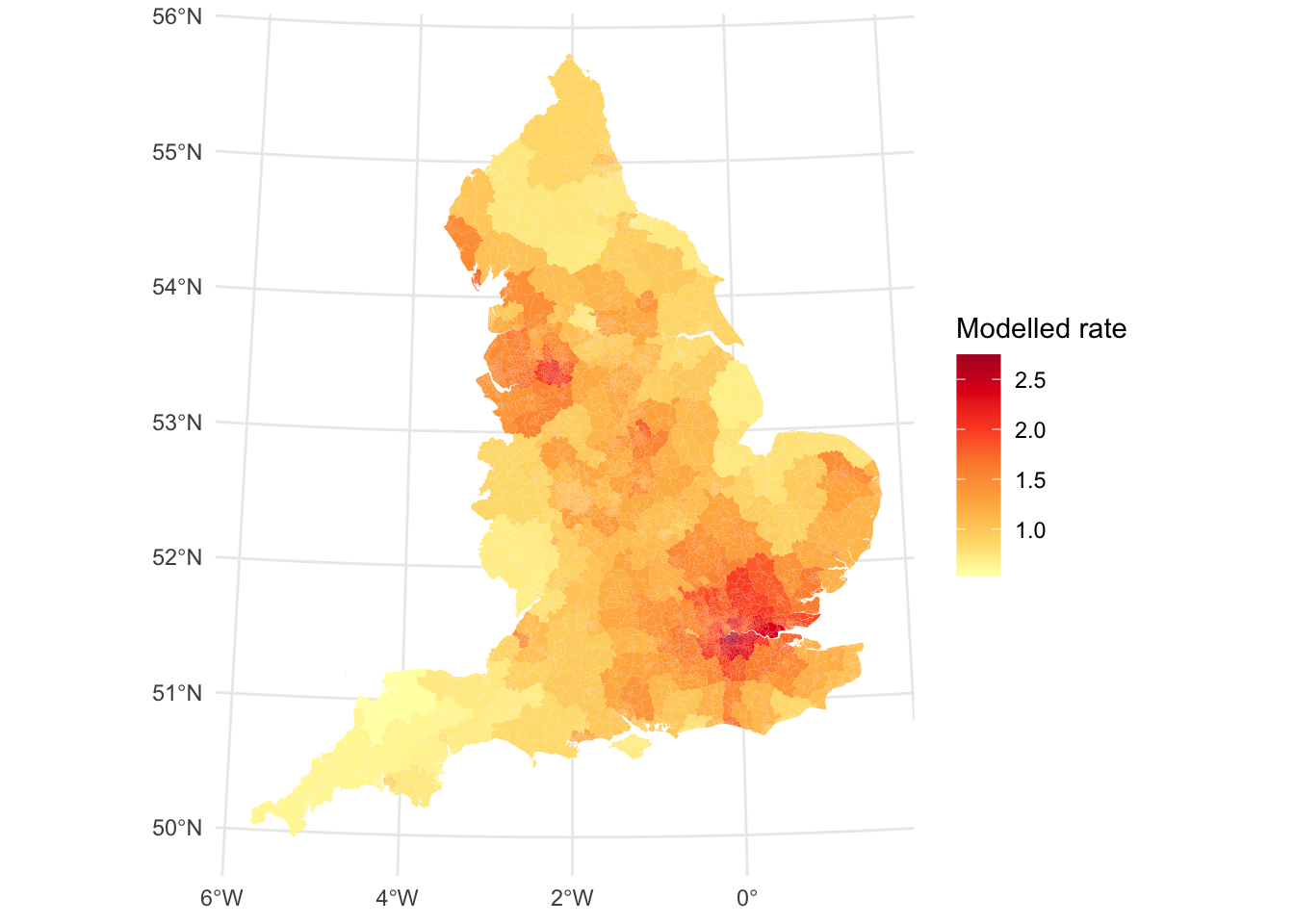
Second, multilevel models can be used – as their name suggests! – to fit multi-level models to examine the scale of the geographic pattern of a variable. Consider the following example, which fits a multilevel model to the COVID-19 rates of all English neighbourhoods in the week before Christmas 2021. There are now three levels in the model, which are the base neighbourhoods level, then the local authorities in which the neighourhoods are located, and then the English regions to which the local authorities belong. Hence, three levels and three simultaneous scales of analysis: neighbourhoods, local authorities and regions. Although the resulting map suffers a little from the ‘invisibility problem’ of some small areas within it, the higher COVID-19 rate in parts of London and the South East is evident (but not solely confined to these regions, as there is also a high rate evident in the North West).
Having fitted a model with three geographic levels, the geographical question that we can now ask is which of the levels of the model contributes most to the geographical patterning of the disease. Do we get most variation between neighbourhoods (suggesting the geographic pattern is mostly at the neighbourhood level), between local authorities (so a local authority patterning) or between regions (evidence of strongest regional differences)? We can answer the question by looking at how much of the variance belongs to each level, which we can see in the summary under Random effects.
Code
summary(mlm)
Linear mixed model fit by REML ['lmerMod']
Formula: rate ~ (1 | LtlaName) + (1 | regionName)
   Data: xmas_covid

REML criterion at convergence: 2858.8

Scaled residuals:
    Min      1Q  Median      3Q     Max
-5.3127 -0.6222 -0.0334  0.5832  6.8771

Random effects:
 Groups     Name        Variance Std.Dev.
 LtlaName   (Intercept) 0.08043  0.2836
 regionName (Intercept) 0.14923  0.3863
 Residual               0.07714  0.2777
Number of obs: 6789, groups:  LtlaName, 315; regionName, 9

Fixed effects:
            Estimate Std. Error t value
(Intercept)     1.26       0.13   9.687
From these summary values we can work out the percentage of the variance which is at each level, calculating what is known as the intraclass correlation (ICC). For this particular week of the pandemic it is,
The ICC appears to suggest the presence of regional effects, in particular (because the ICC for regionName is greater than the ICC for any other level). These regional effects, which are treated as random effects in the model, can be examined using the code below, from which they are found to be strongest for London. This means that the COVID-19 rate for this week is higher for London that it is for any other region.
# A tibble: 9 × 5
  grpvar     term        grp                      condval condsd
  <chr>      <fct>       <fct>                      <dbl>  <dbl>
1 regionName (Intercept) London                    0.814  0.0505
2 regionName (Intercept) East of England           0.236  0.0433
3 regionName (Intercept) North West                0.181  0.0463
4 regionName (Intercept) South East                0.0644 0.0356
5 regionName (Intercept) East Midlands            -0.0688 0.0463
6 regionName (Intercept) West Midlands            -0.189  0.0527
7 regionName (Intercept) Yorkshire and The Humber -0.241  0.0626
8 regionName (Intercept) North East               -0.389  0.0816
9 regionName (Intercept) South West               -0.407  0.0536
Of course, somewhere has to be highest so the fact the it is highest for London does not mean the difference is necessarily statistically significant. However, as it turns out, it is significant (significantly different from zero), which we can see if we plot what is called a caterpillar plot in the multilevel literature, drawn here with a 95% confidence interval around each of the regional effects.
Not only is London’s regional ‘uplift’ in the COVID rates significantly greater than zero, London’s regional effect is greater than for any other regions. The following chart suggests that London is different from the rest because its confidence interval does not overlap with any others. Note that if you are testing to see if two places differ from each other as opposed to from zero then you need to shorten the confidence interval before looking to see if they overlap. As a rule of thumb, the 95% confidence interval for a test of difference in two values is 1.39 \(\times\) the standard error of the parameter estimate instead of the more usual 1.96.
Despite the clear evidence of regional differences that are driven by London’s much higher COVID-19 rate in the week before Christmas 2021, keep in mind that not all the pattern in the COVID-19 rates is at the regional level. To recall,
There are, for example, differences between the local authorities, too, at the next level down in the model. These are evident from a caterpillar plot for the authorities although because there are more of these authorities than there are regions (315 authorities Vs rlength(unique(xmas_covid$regionName))` regions, individual ones are harder to discern.
The key point here is that the multilevel model is useful to help unpack at what scale(s) geographic outcomes are arising and to indentify some of the key places driving those outcomes.
Spatial varying coefficient effects
The mutilevel models fitted above are random intercepts models – only the intercept term is permitted to vary from place to place. Under these models, some places are expected to have a higher or lower average COVID-19 rate than others but that rate is not affected by any predictor variables that can also very in their effects from place-to-place.
Imagine that the percentage of the population of secondary school age is a factor in the COVID-19 rates in London ahead of Christmas 2021. It is a very simple model but it appears to have some (limited) explanatory power. As it happens, more children of school age appears to be less associated with COVID, perhaps because they and the families had already caught it?
Code
ols <-lm(rate ~ age12.17, data = ldn_covid_sp)summary(ols)
Call:
lm(formula = rate ~ age12.17, data = ldn_covid_sp)

Residuals:
     Min       1Q   Median       3Q      Max
-1.11561 -0.29813 -0.00225  0.27856  1.20720

Coefficients:
             Estimate Std. Error t value Pr(>|t|)
(Intercept)  2.629006   0.058593  44.869   <2e-16 ***
age12.17    -0.076615   0.008245  -9.292   <2e-16 ***
---
Signif. codes:  0 '***' 0.001 '**' 0.01 '*' 0.05 '.' 0.1 ' ' 1

Residual standard error: 0.4111 on 980 degrees of freedom
Multiple R-squared:  0.08097,   Adjusted R-squared:  0.08003
F-statistic: 86.34 on 1 and 980 DF,  p-value: < 2.2e-16
A geographically weighted regression suggests that there might be spatial variation in the relationship between age12.17 and the COVID rate. In truth, not all of these local estimates are necessarily significant but let us ignore that for the moment.
(Fit the GWR model allowing for spatial variation in the effects of age12.17 on rate)
Code
require(GWmodel)bw <-bw.gwr(rate ~ age12.17, data = ldn_covid_sp, adaptive =TRUE)
The closest multilevel model to the above GWR model (given the current data) is one that allows the effects of age12.17 to vary by local authority (LtlaName).
(fit the model)
Code
mlm <-lmer(rate ~ (age12.17|LtlaName), data = ldn_covid)
Again, there are commonalities in the GWR and MLM estimates but the differing conceptions of the structure of geographic space and the spatial relationships it contains makes a difference to the results.
More to be added!
This session is incomplete. For now, the key point is that GWR and multilevel models conceptualise space in different ways. I am not meaning to imply that multilevel models are worse, as they can be very useful and flexible. It useful to note that there are now methods that intgrate spatial regression models with multilevel models (see, for example, here and GWR with hierarchical group structures (for example, this and this but these are pretty advanced methods of analysis!
---title: "Continuous and discrete views of the spatial variable"subtitle: "From GWR to multilevel modelling"execute: warning: false message: false---```{r}#| include: falseinstalled <-installed.packages()[,1]required <-c("sf", "tidyverse", "ggplot2", "GWmodel", "lme4")install <- required[!(required %in% installed)]if(length(install)) install.packages(install, dependencies =TRUE, repos ="https://cloud.r-project.org")```(Draft version)## IntroductionGeographically Weighted Regression, which we looked at in the previous session, treats geographic space as a continuous spatial variable in the sense that regression relationships can vary from one location to another across a geographic study region. That continuous view of space is clear if we fit a simple 'null model' of the COVID-19 rates in London in the week before Christmas 2021 and map the results. It is a null model because it includes no predictor variables other than the local estimate of the intercept (i.e. the local mean rate of COVID-19). What is clear is how that local estimate is allowed to vary across geographic space.(Download and extract the data for London and fit the GWR model)```{r}#| results: falserequire(sf)require(ggplot2)require(tidyverse)require(GWmodel)if(!file.exists("covid_xmas_2021.geojson")) download.file("https://github.com/profrichharris/profrichharris.github.io/raw/main/MandM/data/covid_xmas_2021.geojson", "covid_xmas_2021.geojson", mode ="wb", quiet =TRUE)xmas_covid <-read_sf("covid_xmas_2021.geojson")xmas_covid %>%filter(regionName =="London") -> ldn_covidldn_covid_sp <-as_Spatial(ldn_covid)bw <-bw.gwr(rate ~1, data = ldn_covid_sp, adaptive =TRUE)gwrmod <-gwr.basic(rate ~1, data = ldn_covid_sp, bw = bw, adaptive =TRUE)```(Map the predicted COVID-19 rates across London based on the spatially varying local mean estimate)```{r}ldn_covid$yhat <- gwrmod$SDF$yhatggplot(data = ldn_covid, aes(fill = yhat)) +geom_sf(size =0.25) +scale_fill_distiller("Modelled rate", palette ="YlOrRd", direction =1, limits =c(1.2,3)) +theme_minimal()```Multilevel models, by contrast, have more of a discrete view of space because observations at some base level are treated as members of a group at a second, more aggregate level. In a geographic context, the base level could be neighbourhoods and the groups could be the local authorities to which the neighbourhoods belong. This more discrete view of space becomes clear if we fit a very simple (too simple, really) null model of the COVID-19 rates in London, using the local authority estimates from this multilevel model as the nearest equivalent to the local means of the GWR model.```{r}require(lme4)mlm <-lmer(rate ~ (1|LtlaName), data = ldn_covid)ldn_covid$yhat <-predict(mlm, re.form =~ (1|LtlaName))ggplot(data = ldn_covid, aes(fill = yhat)) +geom_sf(size =0.25) +scale_fill_distiller("Modelled rate", palette ="YlOrRd", direction =1, limits =c(1.2,3)) +theme_minimal()```If we compare the map above with that produced from the GWR estimates then we find that there are commonalities in the two maps but the multilevel model clearly has the more bounded view of geographic space.## Multilevel modelsThe package that we are using to fit the models here is [lme4](https://cran.r-project.org/web/packages/lme4/index.html){target="_blank"}. The formula `rate ~ (1|LtlaName)` means that we are modelling the COVID-19 `rate` against a random intercept that varies by local authority (by local authority name, `LtlaName`). It is not the only way of fitting multilevel models in R (an alternative, for example, is [brms](https://cran.r-project.org/web/packages/brms/vignettes/brms_multilevel.pdf){target="_blank"}) but it is sufficient for the purposes of this exercise.The more discrete and bounded view of geographic space that the multilevel model (in its simplest form, at least) employs seems quite restricting -- in this case study it is suggesting that the causes of COVID-19 are somehow related to 'things' that happen or have consequences at a local authority scale. The implication is that the boundaries of local authorities are relevant to the geographical causes and rates of COVID-19. This is not an assumption that GWR makes so why use multilevel models instead?One answer is that a multilevel model is often faster to fit. Consider the following example, which extends the study region to London and the South East.(Fit the GWR model and the multilevel model)```{r}#| results: falsexmas_covid %>%filter(regionName =="London"| regionName =="South East") -> ldn_se_covidldn_se_covid_sp <-as_Spatial(ldn_se_covid)t1 <-Sys.time()bw <-bw.gwr(rate ~1, data = ldn_se_covid_sp, adaptive =TRUE)gwrmod <-gwr.basic(rate ~1, data = ldn_se_covid_sp, bw = bw, adaptive =TRUE)gwrt <-Sys.time() - t1t2 <-Sys.time()mlm <-lmer(rate ~ (1|LtlaName), data = ldn_se_covid)mlmt <-Sys.time() - t2```The computation times are,```{r}gwrtmlmt```Admittedly, neither took very long to fit, with the GWR taking `r round(as.numeric(gwrt, units = "mins"), 2)` minutes and the multilevel model (MLM) taking `r round(as.numeric(mlmt, units = "secs"), 2)` seconds on my laptop. However, these differences become more noticeable with more complex models or larger study regions. The multilevel model is estimating far fewer model parameters than the GWR. This is because the GWR is really lots of models that are fitted separately (one for each location) and then compared, whereas the multilevel model is one model but one which allows for variance at the geographic level(s) of the model, so better local authorities, for example. Put another way, the GWR is a series of local models that are compared, whereas the multilevel model is a global model that allows for local variations around it: at the moment, all it is doing is estimating the average COVID rate for the whole study region but also recognising that different local authorities have rates that vary around the overall average.Second, multilevel models can be used -- as their name suggests! -- to fit multi-level models to examine the scale of the geographic pattern of a variable. Consider the following example, which fits a multilevel model to the COVID-19 rates of all English neighbourhoods in the week before Christmas 2021. There are now three levels in the model, which are the base neighbourhoods level, then the local authorities in which the neighourhoods are located, and then the English regions to which the local authorities belong. Hence, three levels and three simultaneous scales of analysis: neighbourhoods, local authorities and regions. Although the resulting map suffers a little from the 'invisibility problem' of some small areas within it, the higher COVID-19 rate in parts of London and the South East is evident (but not solely confined to these regions, as there is also a high rate evident in the North West).```{r}mlm <-lmer(rate ~ (1|LtlaName) + (1|regionName), data = xmas_covid)xmas_covid$yhat <-predict(mlm, re.form =~ (1|LtlaName) + (1|regionName))ggplot(data = xmas_covid, aes(fill = yhat)) +geom_sf(col =NA) +scale_fill_distiller("Modelled rate", palette ="YlOrRd", direction =1) +theme_minimal()```Having fitted a model with three geographic levels, the geographical question that we can now ask is which of the levels of the model contributes most to the geographical patterning of the disease. Do we get most variation between neighbourhoods (suggesting the geographic pattern is mostly at the neighbourhood level), between local authorities (so a local authority patterning) or between regions (evidence of strongest regional differences)? We can answer the question by looking at how much of the variance belongs to each level, which we can see in the summary under Random effects.```{r}summary(mlm)```From these summary values we can work out the percentage of the variance which is at each level, calculating what is known as the intraclass correlation (ICC). For this particular week of the pandemic it is, ```{r}summary(mlm)$varcor %>% as_tibble %>%select(grp, vcov) %>%mutate(ICC =round(vcov /sum(vcov) *100, 1))```The ICC appears to suggest the presence of regional effects, in particular (because the `ICC` for `regionName` is greater than the ICC for any other level). These regional effects, which are treated as random effects in the model, can be examined using the code below, from which they are found to be strongest for London. This means that the COVID-19 rate for this week is higher for London that it is for any other region. ```{r}ranef(mlm, whichel ="regionName") %>% as_tibble %>%arrange(desc(condval))```Of course, somewhere has to be highest so the fact the it is highest for London does not mean the difference is necessarily statistically significant. However, as it turns out, it is significant (significantly different from zero), which we can see if we plot what is called a caterpillar plot in the multilevel literature, drawn here with a 95% confidence interval around each of the regional effects.```{r}ranef(mlm, whichel ="regionName") %>% as_tibble %>%mutate(lwr = condval -1.96* condsd,upr = condval +1.96* condsd) %>%ggplot(aes(x = grp, y = condval, ymin = lwr, ymax = upr)) +geom_errorbar() +geom_hline(yintercept =0, linetype ="dotted") +theme_minimal() +theme(axis.text.x =element_text(angle =90, vjust =0.5), axis.title.x =element_blank())```Not only is London's regional 'uplift' in the COVID rates significantly greater than zero, London's regional effect is greater than for any other regions. The following chart suggests that London is different from the rest because its confidence interval does not overlap with any others. Note that if you are testing to see if two places differ *from each other* as opposed to from zero then you need to shorten the confidence interval before looking to see if they overlap. As a rule of thumb, the 95% confidence interval for a test of difference in two values is 1.39 $\times$ the standard error of the parameter estimate instead of the more usual 1.96.```{r}ranef(mlm, whichel ="regionName") %>% as_tibble %>%mutate(lwr = condval -1.39* condsd,upr = condval +1.39* condsd) %>%ggplot(aes(x = grp, y = condval, ymin = lwr, ymax = upr)) +geom_errorbar() +theme_minimal() +theme(axis.text.x =element_text(angle =90, vjust =0.5), axis.title.x =element_blank())```Despite the clear evidence of regional differences that are driven by London's much higher COVID-19 rate in the week before Christmas 2021, keep in mind that not all the pattern in the COVID-19 rates is at the regional level. To recall,```{r}summary(mlm)$varcor %>% as_tibble %>%select(grp, vcov) %>%mutate(ICC =round(vcov /sum(vcov) *100, 1))```There are, for example, differences between the local authorities, too, at the next level down in the model. These are evident from a caterpillar plot for the authorities although because there are more of these authorities than there are regions (`r length(unique(xmas_covid$LtlaName))` authorities Vs `r `length(unique(xmas_covid$regionName))` regions, individual ones are harder to discern.```{r}ranef(mlm, whichel ="LtlaName") %>% as_tibble %>%mutate(lwr = condval -1.96* condsd,upr = condval +1.96* condsd) %>%ggplot(aes(x = grp, y = condval, ymin = lwr, ymax = upr)) +geom_errorbar() +geom_hline(yintercept =0, linetype ="dotted") +theme_minimal() +theme(axis.text.x =element_blank()) +xlab("Local authorities")```Looking at the 'top ten' with COVID-19 rates higher than the national and their regional averages would predict are,```{r}ranef(mlm, whichel ="LtlaName") %>% as_tibble %>%arrange(desc(condval)) %>%mutate(lwr = condval -1.96* condsd,upr = condval +1.96* condsd) %>%slice_max(condval, n =10)```The key point here is that the multilevel model is useful to help unpack at what scale(s) geographic outcomes are arising and to indentify some of the key places driving those outcomes.## Spatial varying coefficient effectsThe mutilevel models fitted above are random intercepts models -- only the intercept term is permitted to vary from place to place. Under these models, some places are expected to have a higher or lower average COVID-19 rate than others but that rate is not affected by any predictor variables that can also very in their effects from place-to-place.Imagine that the percentage of the population of secondary school age is a factor in the COVID-19 rates in London ahead of Christmas 2021. It is a very simple model but it appears to have some (limited) explanatory power. As it happens, more children of school age appears to be less associated with COVID, perhaps because they and the families had already caught it?```{r}ols <-lm(rate ~ age12.17, data = ldn_covid_sp)summary(ols)```A geographically weighted regression suggests that there might be spatial variation in the relationship between `age12.17` and the COVID `rate`. In truth, not all of these local estimates are necessarily significant but let us ignore that for the moment.(Fit the GWR model allowing for spatial variation in the effects of `age12.17` on `rate`)```{r}require(GWmodel)bw <-bw.gwr(rate ~ age12.17, data = ldn_covid_sp, adaptive =TRUE)gwrmod <-gwr.basic(rate ~ age12.17, data = ldn_covid_sp, adaptive =TRUE, bw = bw)```(Map the results)```{r}ldn_covid$age12.17GWR <- gwrmod$SDF$age12.17ggplot(data = ldn_covid, aes(fill = age12.17GWR)) +geom_sf(size =0.25) +scale_fill_gradient2(trans ="reverse", limits =c(0.237, -0.282)) +theme_minimal() +guides(fill =guide_colourbar(reverse =TRUE))```The closest multilevel model to the above GWR model (given the current data) is one that allows the effects of `age12.17` to vary by local authority (`LtlaName`).(fit the model)```{r}mlm <-lmer(rate ~ (age12.17|LtlaName), data = ldn_covid)```(plot the results)```{r}ranef(mlm, whichel ="LtlaName") %>% as_tibble %>%filter(term =="age12.17") %>%rename(LtlaName = grp,age12.17LM = condval) %>%select(LtlaName, age12.17LM) %>%inner_join(ldn_covid, ., by ="LtlaName") %>%ggplot(aes(fill = age12.17LM)) +geom_sf(size =0.25) +scale_fill_gradient2(trans ="reverse", limits =c(0.237, -0.282)) +theme_minimal() +guides(fill =guide_colourbar(reverse =TRUE))```Again, there are commonalities in the GWR and MLM estimates but the differing conceptions of the structure of geographic space and the spatial relationships it contains makes a difference to the results.## More to be added!This session is incomplete. For now, the key point is that GWR and multilevel models conceptualise space in different ways. I am not meaning to imply that multilevel models are worse, as they can be very useful and flexible. It useful to note that there are now methods that intgrate spatial regression models with multilevel models (see, for example, [here](http://cran.nexr.com/web/packages/HSAR/index.html){target="_blank"} and GWR with hierarchical group structures (for example, [this](https://onlinelibrary.wiley.com/doi/abs/10.1111/tgis.12020){target="_blank"} and [this](https://journals.sagepub.com/doi/abs/10.1177/23998083211063885){target="blank"} but these are pretty advanced methods of analysis!## Further Reading[Multilevel models](https://www.dropbox.com/s/8zaazt2vsnwtow6/3117-107460_Rey-Franklin_CH10.pdf?dl=1){target="_blank"} -- an introduction to multilevel models from the [Handbook of Spatial Analysis in the Social Sciences](https://www.e-elgar.com/shop/gbp/handbook-of-spatial-analysis-in-the-social-sciences-9781789903935.html){target="_blank"}.