In the previous session we looked at geographically weighted statistics, including geographically weighted correlation, which examines whether the correlation – and therefore the direction and/or the strength of the relationship – between two variables varies across a map. In this session we extend from correlation to looking at regression modelling with a spatial component. This is spatial regression. The data we shall use are a map of the rate of COVID-19 infections per thousand population in neighbourhoods of the North West of England over the period from the week commencing 2020-03-07 to the week commencing 2022-04-16. That rate is calculated as the total number of reported infections per neighbourhood, divided by the mid-2020 ONS estimated population.
The rate, as calculated, does not allow for re-infection (i.e. the same person can catch COVID-19 more than once).
Not everyone who had COVID was tested for a positive diagnosis. Limitations in the testing regime are described in this paper and are most severe earlier in the pandemic and again towards the end of the data period when testing was scaled-back and then largely withdrawn.
For data protection reasons, where a neighbourhood had less than three cases in a week, that number was reported as zero even though it could really be one or two. This undercount adds up, although, unsurprisingly it affects the largest cities most (because they have more neighbourhoods to be undercounted) in weeks when COVID is not especially prevalent (because in other weeks there are more often more than two cases per neighbourhoods). An adjustment has been made to the data to allow for this censoring of the data but not for the undercount caused by not testing positive.
Despite their shortcomings, the data are sufficient to illustrate the methods, below.
Getting Started
The data are downloaded as follows. The required packages should be installed already, from previous sessions. As before, you may wish to begin by opening the R Project that you created for these classes.
Code
installed <-installed.packages()[,1]pkgs <-c("sf", "tidyverse", "ggplot2", "spdep", "GWmodel")install <- pkgs[!(pkgs %in% installed)]if(length(install)) install.packages(install, dependencies =TRUE)if(!("ggsflabel"%in% installed)) remotes::install_github("yutannihilation/ggsflabel")require(sf)require(tidyverse)require(ggplot2)require(ggsflabel)if(!file.exists("covid.geojson")) download.file("https://github.com/profrichharris/profrichharris.github.io/raw/main/MandM/data/covid.geojson","covid.geojson", mode ="wb", quiet =TRUE)read_sf("covid.geojson") |>filter(regionName =="North West") -> covid# The step below is just to reformat some of the names of the data variables,# replacing age0-11 with age0.11, age12_17 with age 12.17, and so forth.names(covid) <-sub("-", "\\.", names(covid))
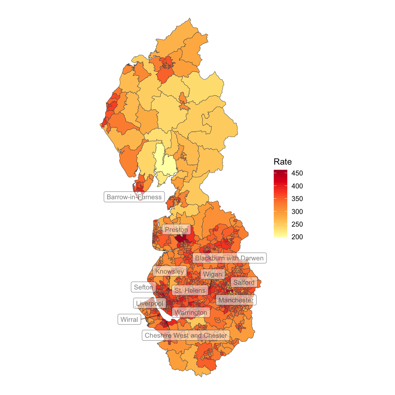
Looking at a map of the COVID-19 rates, it appears that there are patches of higher rates that tend to cluster in cities such as Preston, Manchester and Liverpool, although not exclusively so.
Don’t forget that you can, if you wish, use the cols4all and it’s functions, e.g. scale_fill_continuous_c4a_seq() instead of scale_fill_distiller() in the code chunk below.
Code
covid |>filter(Rate >400) |>select(LtlaName) |># LtlaName is the name of the local authorityfilter(!duplicated(LtlaName)) -> high_rateggplot() +geom_sf(data = covid, aes(fill = Rate), size =0.25) +scale_fill_distiller(palette ="YlOrRd", direction =1) +geom_sf_label_repel(data = high_rate, aes(label = LtlaName), size =3,alpha =0.5) +theme_void()
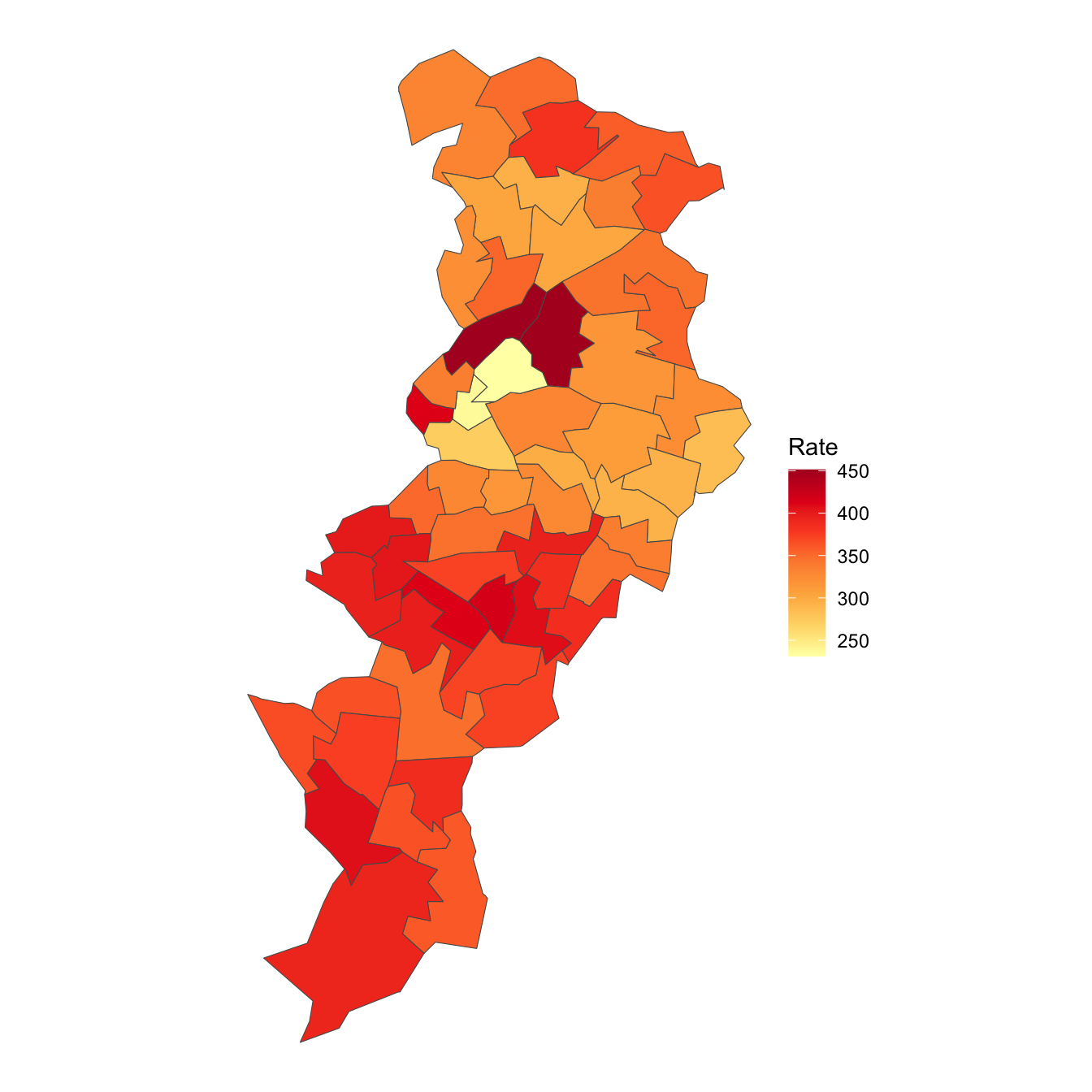
… and with variation within the cities such as Manchester:
Across the map there appears to be a pattern of positive spatial autocorrelation in the COVID-19 rates of contiguous neighbours (‘hot spots’), as evident using a Moran test,
    Moran I test under randomisation

data:  covid$Rate
weights: spweight

Moran I statistic standard deviate = 24.422, p-value < 2.2e-16
alternative hypothesis: greater
sample estimates:
Moran I statistic       Expectation          Variance
     0.4919206758     -0.0010834236      0.0004075223
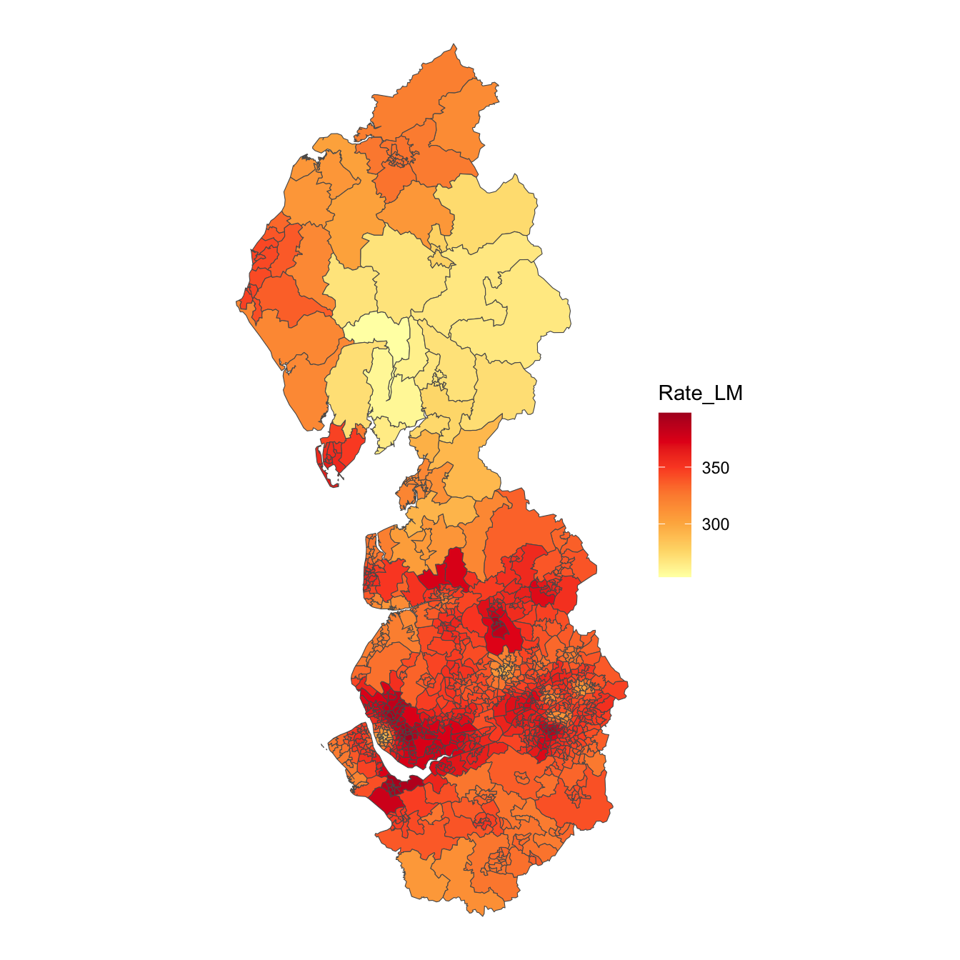
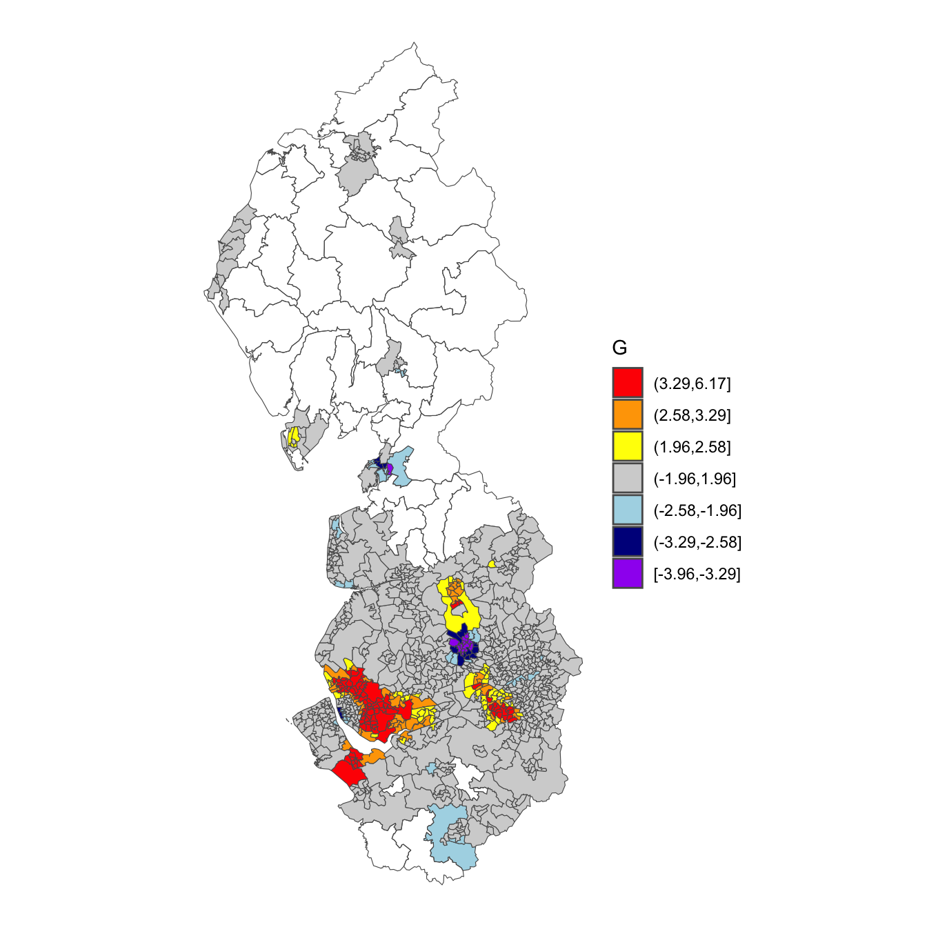
Some of the ‘hot spots’ of infection are suggested using the geographically-weighted means,
An initial model to explain the spatial patterns in the COVID-19 rates
It is likely that the spatial variation in the COVID-19 rates is due to differences in the physical attributes of the different neighbourhoods and/or of the populations who live in them. For example, the rates may be related to the relative level of deprivation in the neighbourhoods (the Index of Multiple Deprivation, IMD), the age composition of their populations (e.g. percentage aged 0 to 11, age0.11), the population density (density), the number of carehome beds (carebeds, because particularly early on in the pandemic, carehome residents were at very high risk), and whether they contain an Accident and Emergency hospital (AandE, coded 1 if they do and 0 if they don’t). Incorporating this into a standard regression model gives,
which, as its R-squared value of 0.204 suggests, goes some way to explaining the variation in the rates. Note that you can tidier output for some models using tidyvere’s broom package and functions.
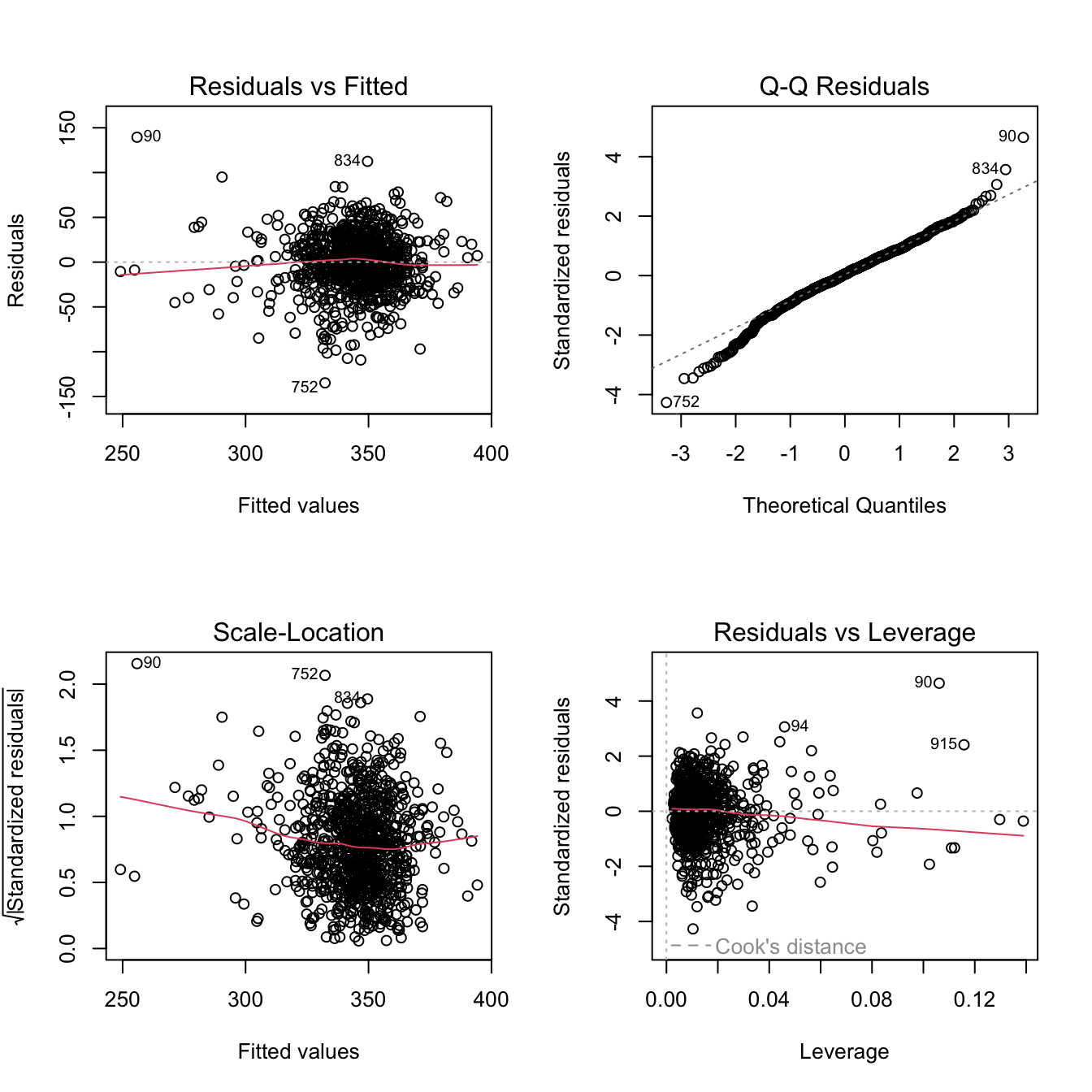
Looking at R’s standard diagnostic plots there is not any strong evidence that the standard residual Normality assumption of the regression statistics is being violated although, not very surprisingly, the variance inflation values (VIF) do suggest high levels of colinearity between the age variables.
There are no hard and fast rules but, in broad terms, a VIF value of 4 or 5 or above is worth considering as a potential issue and a value above 10 suggests a very high level of multicollinearity. The simple solution to the issue is to drop some of the colinear variables but not all: if X1 and X2 are highly correlated, you only need to consider dropping X1 or X2, not both.
Although I am generally cautious about automated selection procedures, in this case a stepwise model selection appears useful to address the colinearity:
An analysis of variance (ANOVA) shows there is no statistically gain in using the model with more variables (ols1) so we can prefer the simpler (ols2).
Code
anova(ols2, ols1)
Analysis of Variance Table

Model 1: Rate ~ IMD + age0.11 + age25.34 + age35.39 + age50.59 + carebeds
Model 2: Rate ~ IMD + age0.11 + age12.17 + age18.24 + age25.34 + age35.39 +
    age50.59 + age60.69 + age70plus + density + carebeds + AandE
  Res.Df    RSS Df Sum of Sq      F Pr(>F)
1    917 921337
2    911 918176  6    3161.6 0.5228 0.7913
Looking again at the model (tidy(ols2)), it may seem surprising that the deprivation index is negatively correlated with the COVID rate – implying more deprivation, fewer infections (geographies of health often work in the opposite direction; being poorer can come with a ‘health premium’) – but this is due to the later variants of the disease that spread quickly through more affluent populations when restrictions on mobility and social interaction have been relaxed.
Spatial dependencies in the model residuals
Although the model appears to fit the data reasonably well, there is a problem. The residuals – the differences between what the model predicts as the COVID-19 rate at each location and what those rates actually are – are supposed to be random noise, meaning their values should be independent of their location and of each other, with no spatial structure. They are not. In fact, if we apply a Moran’s test to the residuals, using the test for regression residuals, lm.morantest(), we find that they are significantly spatially correlated:
Code
lm.morantest(ols2, spweight)
    Global Moran I for regression residuals

data:
model: lm(formula = Rate ~ IMD + age0.11 + age25.34 + age35.39 +
age50.59 + carebeds, data = covid)
weights: spweight

Moran I statistic standard deviate = 22.357, p-value < 2.2e-16
alternative hypothesis: greater
sample estimates:
Observed Moran I      Expectation         Variance
    0.4461249282    -0.0033794098     0.0004042296
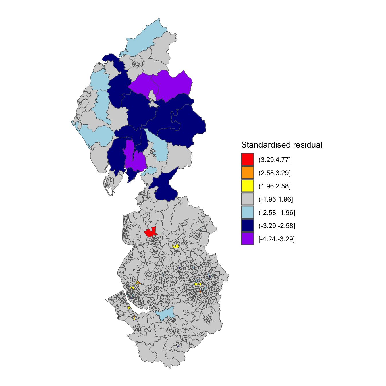
The pattern is evident if we map the standardised residuals from the function rstandard(). At the risk of geographic over-simplification, there is something of a north-south divide, with a patch of negative residuals to the north of the study region. These are rural neighbouhoods where the model is under-predicting the rate of COVID-19 cases.
It is possible that the spatial structure in the residuals exists because the model has been mis-specified. In particular, we might wonder if it was a mistake to drop the population density variable which perhaps had a polynomial (non-linear) relationship with the COVID rates. Let’s find out.
Code
ols3 <-update(ols2, . ~ . +poly(density, 2))
Certainly, of the three models, this is the best fit to the data, as we can see from the various model fit diagnostics that are easily gathered together using the glance() function. Note the highest, adjusted r-squared value and lowest AIC value, for example.
One way to handle the error structure is to fit a spatial simultaneous autoregressive error model which decomposes the error (the residuals) into two parts: a spatially lagged component (the bit that allows for geographical clustering in the residuals) and a remaining error: \(y = X\beta + \lambda W \xi + \epsilon\). The model can be fitted using R’s spatialreg package.
Call:errorsarlm(formula = formula(ols3), data = covid, listw = spweight)

Residuals:
     Min       1Q   Median       3Q      Max
-88.9057 -13.5631   1.0775  15.1597 108.7168

Type: error
Coefficients: (asymptotic standard errors)
                     Estimate  Std. Error z value  Pr(>|z|)
(Intercept)        228.423021   13.194612 17.3118 < 2.2e-16
IMD                 -0.595478    0.089535 -6.6508 2.915e-11
age0.11              1.885127    0.449453  4.1943 2.738e-05
age25.34             2.612570    0.416075  6.2791 3.406e-10
age35.39             3.729977    1.369957  2.7227  0.006475
age50.59             3.339295    0.608468  5.4880 4.064e-08
carebeds             0.051339    0.010181  5.0426 4.592e-07
poly(density, 2)1 -111.989456   38.123934 -2.9375  0.003309
poly(density, 2)2 -120.005358   28.931984 -4.1478 3.356e-05

Lambda: 0.69751, LR test value: 348.94, p-value: < 2.22e-16
Asymptotic standard error: 0.028893
    z-value: 24.142, p-value: < 2.22e-16
Wald statistic: 582.82, p-value: < 2.22e-16

Log likelihood: -4298.755 for error model
ML residual variance (sigma squared): 572.93, (sigma: 23.936)
Number of observations: 924
Number of parameters estimated: 11
AIC: 8619.5, (AIC for lm: 8966.5)
The spatial component, \(\lambda\), the spatial autocorrelation in the residuals, is significant as a number of test statistics that are with it in the summary above show. What it confirms is what we could interpret from the earlier Moran’s test of the regression residuals: having allowed for the variables that help to predict the COVID-rates there is still an unexplained geographic pattern whereby places for which the model over-predict the rate tend to be surrounded by other places where it does the same, and places where it under-predicts are surrounded by other under-predictions. The spatial error model gives a better fit to the data than the standard regression, as the following diagnostics tell us (the lower the AIC the better)
Code
glance(ols3)$r.squared
[1] 0.2479886
Code
glance(errmod)$r.squared
[1] 0.5543411
Code
AIC(ols3)
[1] 8966.455
Code
AIC(errmod)
[1] 8619.511
The differences are such that there is little doubt that the error model offers a much improved fit but if we do wish to test that difference statistically then
For example, where the estimate for age50.59, which is the estimate of the effect size, used to be 5.67, now it is 3.34. The 95% confidence intervals for those and the other coefficient estimates change too:
Although the spatial error model fits the data better than the standard regression model, it tells us only that there is an unexplained spatial structure to the residuals, not what caused it. It may offer better estimates of the model parameters and their statistical significance but it does not presuppose any particular spatial process generating the patterns in the values. A different model that explicitly tests for whether the value at a location is functionally dependent on the values of neighbouring location is the spatially lagged y model: \(y = \rho Wy + X\beta + \epsilon\). It models an ‘overspill’ or chain effect where the outcome (the Y value) at any location is affected by the outcomes at surrounding locations.
Code
lagmod <-lagsarlm(formula(ols3), data = covid, listw = spweight)summary(lagmod)
Call:lagsarlm(formula = formula(ols3), data = covid, listw = spweight)

Residuals:
     Min       1Q   Median       3Q      Max
-98.8140 -14.8770   1.0467  14.7420 110.1081

Type: lag
Coefficients: (asymptotic standard errors)
                     Estimate  Std. Error z value  Pr(>|z|)
(Intercept)         17.353050   14.403449  1.2048 0.2282866
IMD                 -0.371501    0.074903 -4.9598 7.057e-07
age0.11              1.377790    0.411239  3.3503 0.0008071
age25.34             2.678105    0.367344  7.2905 3.089e-13
age35.39             1.885234    1.235376  1.5260 0.1269996
age50.59             3.636195    0.553621  6.5680 5.099e-11
carebeds             0.042747    0.010887  3.9264 8.623e-05
poly(density, 2)1  -69.714325   34.062239 -2.0467 0.0406900
poly(density, 2)2 -156.910145   28.073145 -5.5893 2.279e-08

Rho: 0.63167, LR test value: 342.73, p-value: < 2.22e-16
Asymptotic standard error: 0.02966
    z-value: 21.297, p-value: < 2.22e-16
Wald statistic: 453.57, p-value: < 2.22e-16

Log likelihood: -4301.863 for lag model
ML residual variance (sigma squared): 591.59, (sigma: 24.323)
Number of observations: 924
Number of parameters estimated: 11
AIC: 8625.7, (AIC for lm: 8966.5)
LM test for residual autocorrelation
test value: 3.5747, p-value: 0.058666
Its test for residual autocorrelation does not generate a statistically significant result at a 95% level, meaning there is no statistically significant spatial structure now left in the residuals, although it is close.
Note that the beta estimates of the lagged y-model cannot be interpreted in the same way as for a standard regression model. For example, the beta estimate of -0.372 for the IMD variable does not mean that if (hypothetically) we increased that variable by one unit at each location we should then expect the COVID-19 to everywhere decrease by 0.372 holding the other X variables constant. That is the correct interpretation for a standard (OLS) regression model and also for the spatial error model but not for where the lag of the Y variable is included as a predictor variable. The reason is because if we did raise the IMD value it would start something akin to a ‘chain reaction’ through the feedback of Y via the lagged Y values: the (hypothetical) increase in deprivation at the one location, decreases the COVID-19 rate at neighbouring locations, which decrease the rate at their neighbours and so forth. The total impact is a sum of the direct effect – that predicted to happen through the 1 unit change in IMD – and the indirect effect, which is that caused by ‘the chain reaction’ / feedback / ‘overspill’ in the system:
Although it wasn’t especially noticeable, there was a short pause as those impacts were calculated. The calculations could take much longer if the size of the spatial weights matrix was larger. As this author notes, after Lesage and Pace, 2009, a faster approximation method can be used, here with R = 1000 simulated distributions for the impact measures.
Code
W <-as(spweight, "CsparseMatrix")trMC <-trW(W, type ="MC")im <-summary(impacts(lagmod, tr = trMC, R =1000), zstats =TRUE)data.frame(im$res, row.names =names(lagmod$coefficients)[-1])
In fact, an increase of 1 unit in, for example, the IMD variable, will play out slightly differently in different places because they have different neighbours with different Y values and are at different distances from each other. The code below, which is from the first edition of Ward & Gleditsch (2008, pp.47), will calculate the impact (of a one unit change in IMD) at each location but below I have limited it to the first ten so that it doesn’t take too long to run.
Choosing between the spatial error and lagged y model
Before fitting the spatial error and lagged y models, we could have looked for evidence in support of them using the function lm.LMtests(). This tests the basic OLS specification against the more general spatial error and lagged y models. Anselin and Rey (2014, p.110) offer the following decision tree that can, in the absence of a more theoretical basis for the model choice (e.g. the type of process being modelled), be used in conjunction with the test results to help select the model.
Moving on to the robust tests, only the LM-Lag test is significant. Given the nature of COVID-19 as an infectious disease, it does seem reasonable to suppose that high rates of infection in any an area will ‘overspill’ into neighbouring areas too.
As with the tests of spatial autocorrelation in an earlier session and as with the geographically weighted statistics, the results of the spatial regression models are dependent on the specification of the spatial weights matrix which can suffer from being somewhat arbitrary. We could, if we wish, try calibrating it around the geographically weighted mean.
Code
require(GWmodel)bw <-bw.gwr(Rate ~1, data = covid_sp, adaptive =TRUE, kernel ="bisquare")
To now create the corresponding inverse distance spatial weights matrix for the models, we can use the nn2 function in the RANN package to find the $bw = $ 18 nearest neighbours to each centroid point:
Code
if(!("RANN"%in%installed.packages()[,1])) install.packages("RANN")require(RANN)coords <-st_coordinates(st_centroid(st_geometry(covid)))knn <-nn2(coords, coords, k = bw)
Having done so, those neighbours can be geographically weighted using a bisquare kernel, as in the GWR calibration above. (A Gaussian kernel is obtained if (1 - (x / max(x))^2)^2 is replaced by exp(-0.5 * (x / max(x))^2) in the code below).
Code
d <- knn$nn.distsglist <-apply(d, 1, \(x) { (1- (x /max(x))^2)^2}, simplify =FALSE)knearnb <-knn2nb(knearneigh(st_centroid(st_geometry(covid)), k = bw))spweightK <-nb2listw(knearnb, glist, style ="C")
The results are not very successful though. The lag model with contiguous spatial weights fits the data better,
Code
lagmod3 <-lagsarlm(formula(ols4), data = covid, listw = spweightK)bind_rows(glance(lagmod2), glance(lagmod3))
In addition, the inverse distance weights are not row-standardised, which may cause some knock-on problems. They could become row-standardised (spweightK <- nb2listw(knearnb, glist, style = "W")) but if they are, by re-scaling each row of the weights to equal one, then the inverse distance weighting is altered.
Geographically Weighted Regression
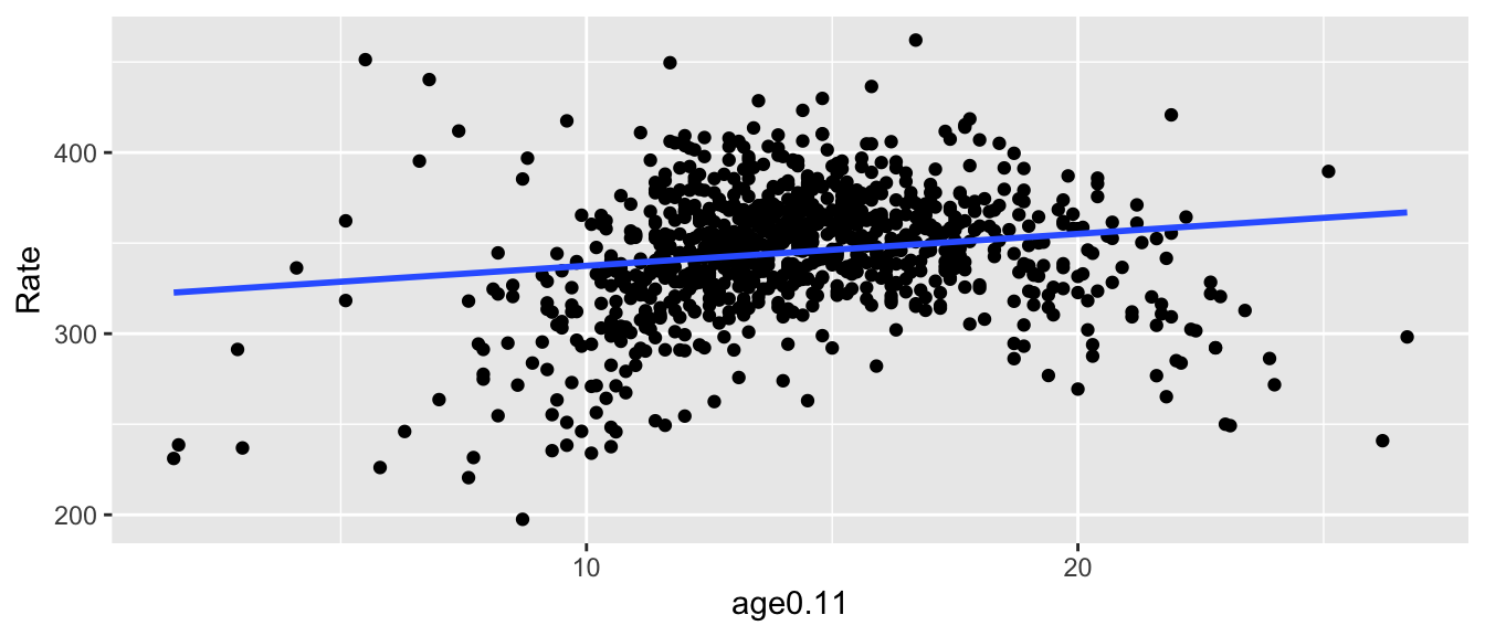
The following charts shows the simple, bivariate regression relationship between Rate and age0.11.
Code
ggplot(covid, aes(x = age0.11, y = Rate)) +geom_point() +geom_smooth(method ="lm", se =FALSE)
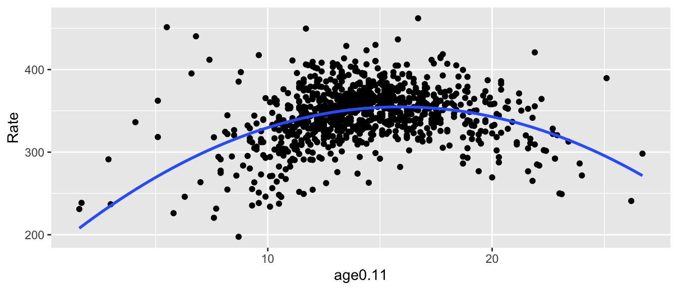
Intriguingly, it doesn’t seem to be linear relationship but a polynomial one.
Code
ggplot(covid, aes(x = age0.11, y = Rate)) +geom_point() +geom_smooth(method ="lm", se =FALSE, formula = y ~poly(x, 2))
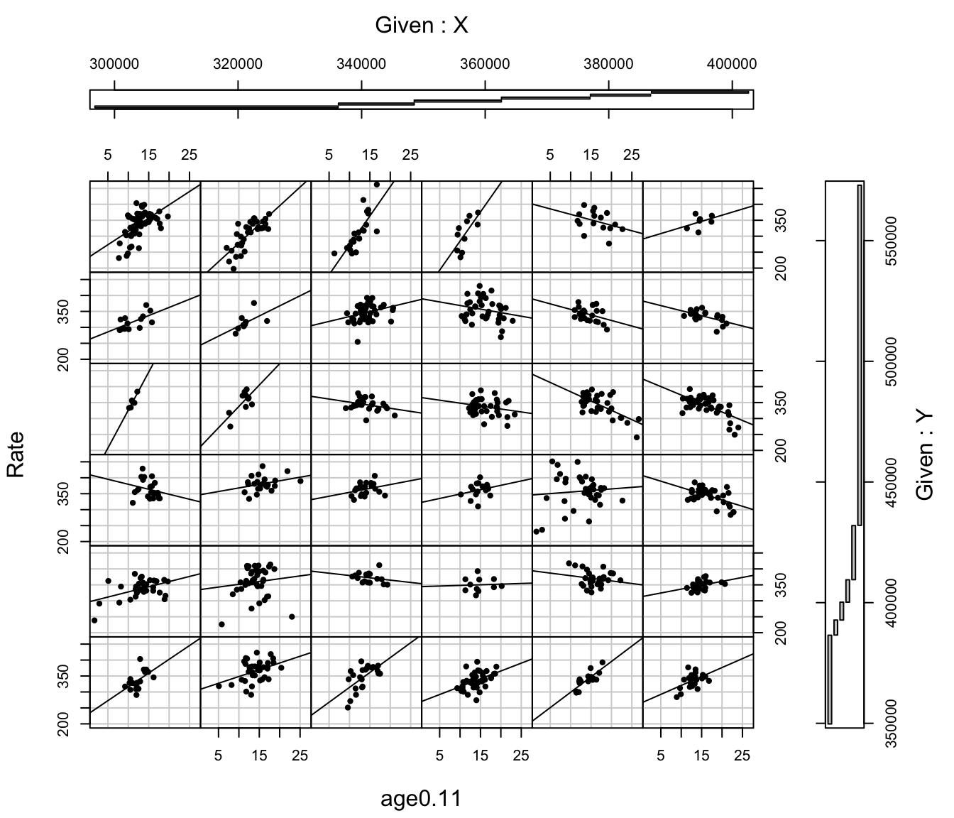
It could be that the relationship is indeed curved but it might also be that the nature of the relationship is spatially dependent – that the relationship between Rate and age0.11 depends upon where it is measured. A coplot() from R’s base graphics lends weight to the second idea: note how the regression relationship changes with X and Y, which are the centroids of the neighbourhoods in the North West of England.
Code
coplot_df <-data.frame(st_coordinates(st_centroid(covid)), Rate = covid$Rate, age0.11 = covid$age0.11)PointsWithLine =function(x, y, ...) {points(x=x, y=y, pch=20, col="black")abline(lm(y ~ x))}coplot(Rate ~ age0.11| X * Y, data = coplot_df, panel = PointsWithLine, overlap =0)
Imagine, now, that instead of dividing the geography of the North West’s neighbourhoods into a \(6 \times 6\) grid, as in the coplot, we instead go from location to location within the study region, calculating a geographically weighted regression at and around each one of them. This builds on the idea of geographically weighted statistics that allow the measured value of the statistic to vary locally from location to location across the study region; with geographically weighted it is the locally estimated regression coefficients that are allowed to vary. These are used to look for spatial variation in the regression relationships.
If the bandwidth is not known or there is no theoretical justification for it, it can be found using an automated selection procedure, here with a more complex model than the bivariate relationship shown in the coplot, instead using all the variables included in the choice between the spatial error and lagged y model, above.
Code
require(GWmodel)bw <-bw.gwr(formula(ols4), data = covid_sp, adaptive =TRUE)
The model can then be fitted.
Code
gwrmod <-gwr.basic(formula(ols4), data = covid_sp, adaptive =TRUE, bw = bw)gwrmod
   ***********************************************************************
   *                       Package   GWmodel                             *
   ***********************************************************************
   Program starts at: 2025-11-23 14:49:32.953047
   Call:
   gwr.basic(formula = formula(ols4), data = covid_sp, bw = bw,
    adaptive = TRUE)

   Dependent (y) variable:  Rate
   Independent variables:  IMD age0.11 age25.34 age50.59 carebeds density
   Number of data points: 924
   ***********************************************************************
   *                    Results of Global Regression                     *
   ***********************************************************************

   Call:
    lm(formula = formula, data = data)

   Residuals:
     Min       1Q   Median       3Q      Max
-123.194  -18.380    1.473   20.623  127.554

   Coefficients:
                       Estimate Std. Error t value Pr(>|t|)
   (Intercept)        188.50375   15.17560  12.422  < 2e-16 ***
   IMD                 -0.39649    0.09149  -4.334 1.63e-05 ***
   age0.11              2.30191    0.41777   5.510 4.66e-08 ***
   age25.34             3.93517    0.34898  11.276  < 2e-16 ***
   age50.59             5.80810    0.69596   8.345 2.59e-16 ***
   carebeds             0.02904    0.01382   2.101   0.0359 *
   poly(density, 2)1   29.14870   43.19300   0.675   0.4999
   poly(density, 2)2 -292.74904   34.12420  -8.579  < 2e-16 ***

   ---Significance stars
   Signif. codes:  0 '***' 0.001 '**' 0.01 '*' 0.05 '.' 0.1 ' ' 1
   Residual standard error: 30.88 on 916 degrees of freedom
   Multiple R-squared: 0.2427
   Adjusted R-squared: 0.2369
   F-statistic: 41.93 on 7 and 916 DF,  p-value: < 2.2e-16
   ***Extra Diagnostic information
   Residual sum of squares: 873446.4
   Sigma(hat): 30.77887
   AIC:  8970.975
   AICc:  8971.172
   BIC:  8151.892
   ***********************************************************************
   *          Results of Geographically Weighted Regression              *
   ***********************************************************************

   *********************Model calibration information*********************
   Kernel function: bisquare
   Adaptive bandwidth: 80 (number of nearest neighbours)
   Regression points: the same locations as observations are used.
   Distance metric: Euclidean distance metric is used.

   ****************Summary of GWR coefficient estimates:******************
                            Min.     1st Qu.      Median     3rd Qu.     Max.
   Intercept         -3.9934e+01  1.3693e+02  2.1422e+02  2.6180e+02 419.5064
   IMD               -2.7499e+00 -7.8059e-01 -4.4223e-01 -1.6702e-01   0.6501
   age0.11           -4.0541e+00  2.3759e-01  3.4220e+00  6.1701e+00  12.5921
   age25.34          -3.9387e+00  1.6469e+00  2.6274e+00  4.2843e+00  13.8157
   age50.59          -9.5346e+00  2.1727e+00  5.3255e+00  8.6233e+00  14.3515
   carebeds          -5.6126e-02  2.5983e-02  5.8662e-02  8.7463e-02   0.2220
   poly(density, 2)1 -2.7204e+03 -4.1814e+02 -1.5602e+02  4.1180e-01 667.9061
   poly(density, 2)2 -2.1980e+03 -5.4619e+02 -2.5300e+02 -1.2247e+02 643.0451
   ************************Diagnostic information*************************
   Number of data points: 924
   Effective number of parameters (2trace(S) - trace(S'S)): 270.2441
   Effective degrees of freedom (n-2trace(S) + trace(S'S)): 653.7559
   AICc (GWR book, Fotheringham, et al. 2002, p. 61, eq 2.33): 8552.959
   AIC (GWR book, Fotheringham, et al. 2002,GWR p. 96, eq. 4.22): 8216.682
   BIC (GWR book, Fotheringham, et al. 2002,GWR p. 61, eq. 2.34): 8513.32
   Residual sum of squares: 313860.8
   R-square value:  0.7278617
   Adjusted R-square value:  0.6151951

   ***********************************************************************
   Program stops at: 2025-11-23 14:49:33.317342
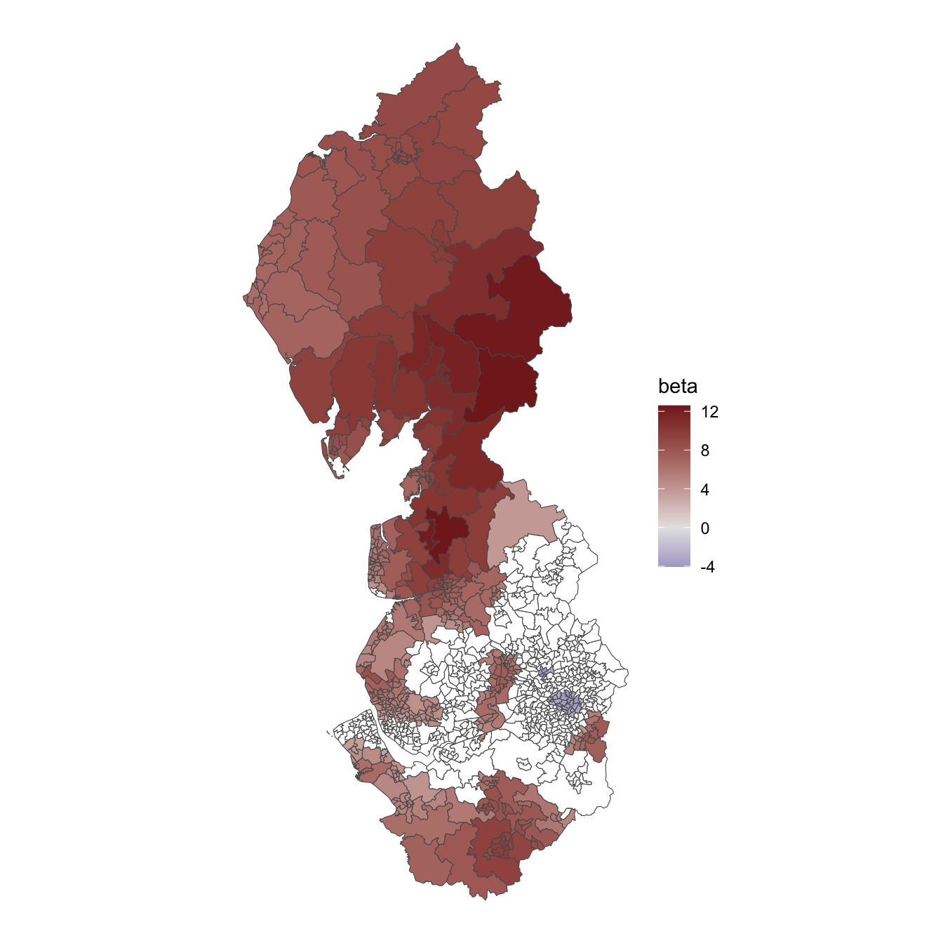
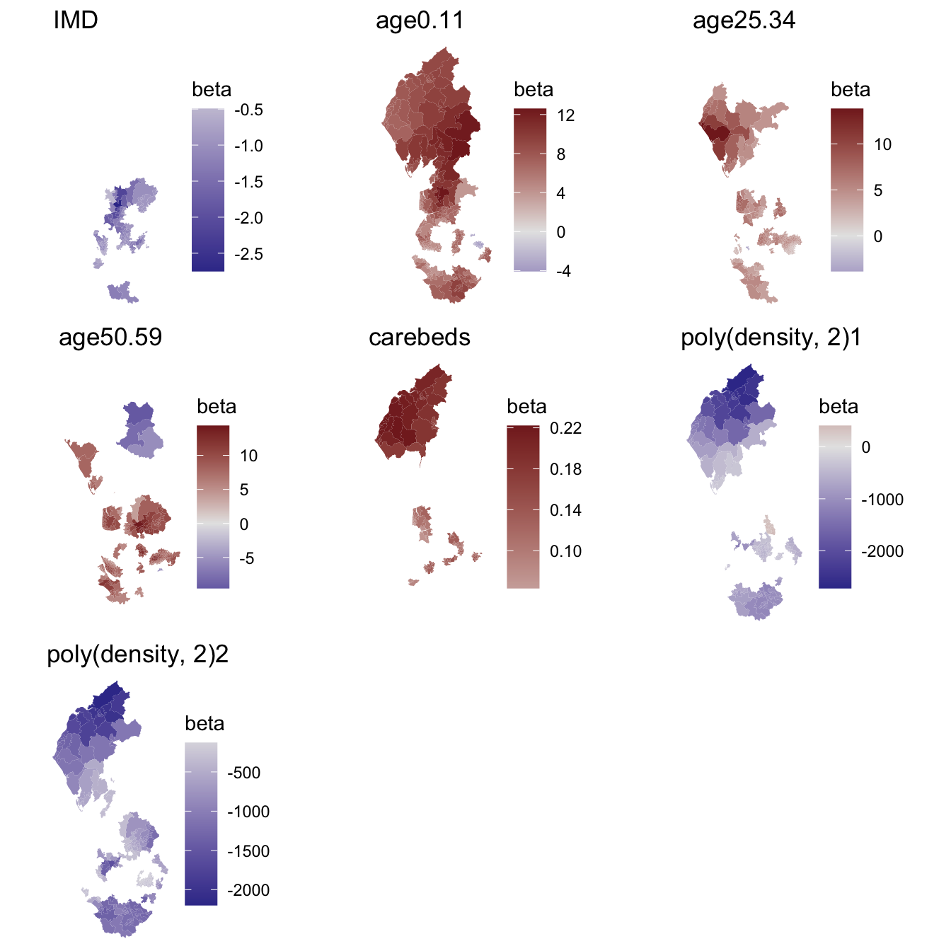
The output requires some interpretation! The results of the global regression are those obtained from a standard OLS regression (i.e. summary(lm(formula(ols4), data = covid_sp))). It is ‘global’ because it is a model for the entire study region, without spatial variation in the regression estimates. The results of the geographically weighted regression are the results from, in this case, 924 separate but spatially overlapping regression models fitted, with geographic weighting, to spatial subsets of the data. All the local estimates are contained in the spatial data frame, gwrmod$SDF, including those for age0.11 which are in gwrmod$SDF$age0.11 and have the following distribution,
Code
summary(gwrmod$SDF$age0.11)
   Min. 1st Qu.  Median    Mean 3rd Qu.    Max.
-4.0541  0.2376  3.4220  3.3645  6.1701 12.5921
This is the same summary of the distribution that is included in the GWR coefficient estimates. What it means is that in at least one location the relationship of age0.11 to Rate is, conditional on the other variables, negative. It is more usual for it to be positive – more children, more infections (perhaps a school effect?) – but the estimated effect size varies quite substantially across the locations in the study region. Its interquartile range is from 0.238 to 6.17. Mapping these local estimates reveals an interesting geography – it is largely in and around Manchester where a greater number of children of primary school age or younger appears to lower instead of raising the infection rate.
… however, not all of these regression estimates are necessarily statistically significant. If we use the estimated t-values to isolate those that are not (t-values less than -1.96 or greater than +1.96 can be considered significant at a 95% confidence), then, for the age0.11 variable we obtain,
I am sure there is a more elegant way of doing this. Don’t worry about the code especially - the point is that not every estimate, everywhere, is significant.
As with the basic GW statistics, we can undertake a randomisation test to suggest whether the spatial variation in the coefficient estimates is statistically significant. However this takes some time to run – with the default nsims = 99 simulations it took about 12 minutes on my laptop. I have ‘commented it out’ in the code block below with the suggestion that you don’t run it now.
Code
# I suggest you do not run this# gwr.mc <- gwr.montecarlo(formula(ols4), covid_sp, adaptive = TRUE, bw = bw)
Instead, let’s jump straight to the results, which I have saved in a pre-prepared workspace.
I suggest you just read over this section rather than do it because it takes some time to run
It appears that only the age0.11 and density variables exhibit significant spatial variation (p-value < 0.05). In principle it is possible to drop the other variables out from the local estimates and treat them as fixed, global estimates instead, in a Mixed GWR model (mixed global and local regression estimates). In the past it has generated an error for me but maybe it will work now?
Code
# This appears to generate an errorgwrmixd <-gwr.mixed(Rate ~ IMD + age0.11+ age25.34+ age50.59+ carebeds +poly(density, 2),data = covid_sp,fixed.vars =c("IMD", "age25.34", "age50.59", "carebeds"),bw = bw, adaptive =TRUE)
If it does not work, We can work around it, using partial regressions, regressing Rate, age0.11 and poly(density, 2) on the fixed variables and using their residuals.
It is also possible to fit a Multiscale GWR, which allows for the possibility of a different bandwith for each variable – see ?gwr.multiscale. Since there is no particular reason to presume that the bandwidth should be the same for all the variables, arguably Multiscale GWR should be preferred over standard GWR, at least in the first instance. Its main drawback, however, is that it takes a while to run – over 3 hours for the code chunk below! (In principle it can be parallelised but it generated an error for me when I tried this with parallel.method = cluster.)
Code
density.1<-poly(covid$density, 2)[, 1]density.2<-poly(covid$density, 2)[, 2]# Do not run!# Took over 3 hours!#gwrmulti <- gwr.multiscale(Rate ~ IMD + age0.11 + age25.34 + age50.59 + carebeds +# density.1 + density.2, data = covid_sp, adaptive = TRUE)
To save time, the results are available below. The bandwidths do appear to vary.
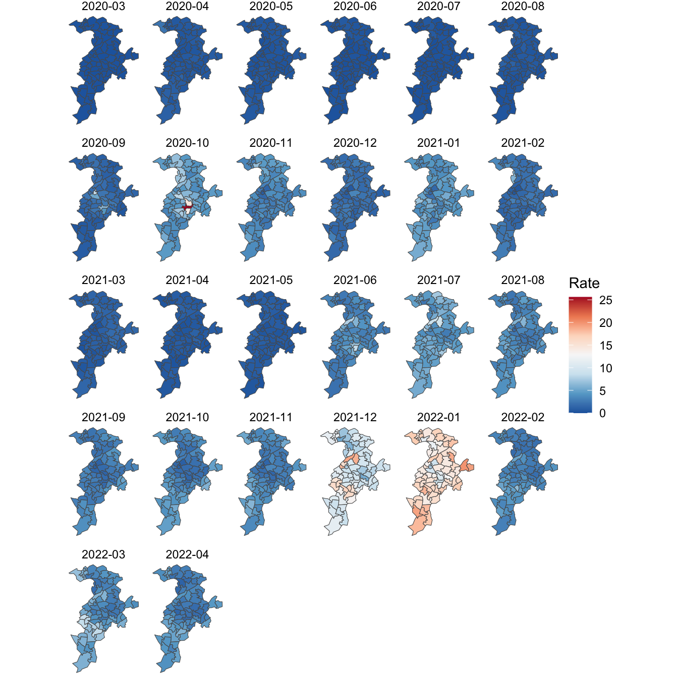
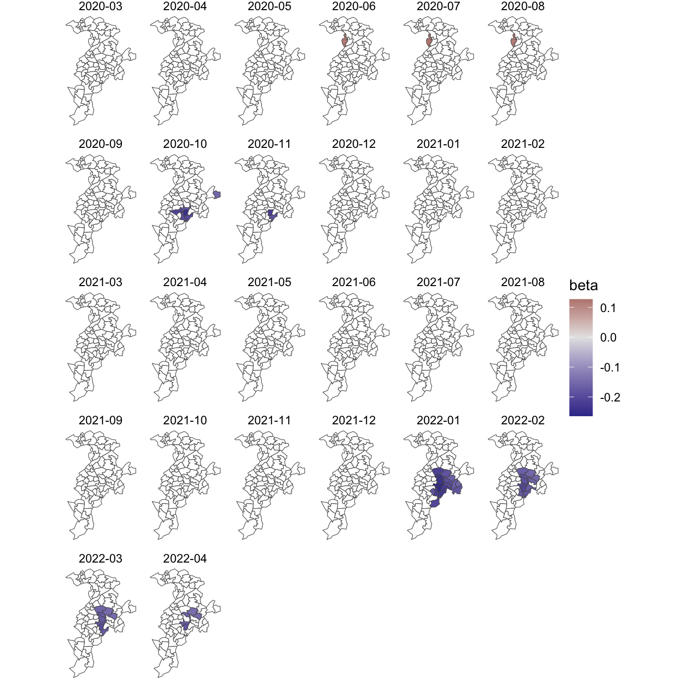
It also possible to add a time dimension and undertake geographically and temporally weighted regression in GWmodel. The following workspace loads monthly COVID-19 data for Manchester neighbourhoods.
If now want to explore how the regression relationships vary in space-time then we can use the bw.gtwr() and gtwr() functions, for which we also need to specify a vector of time tags (obs.tv = ...). In these data, they are simply a numeric value, covid$month_code but see ?bw.gtwr() and ?gtwr() for further possibilities and for further information about the model.
The model will take a little time to run – enough time for you to get a cup of tea or coffee!
   ***********************************************************************
   *                       Package   GWmodel                             *
   ***********************************************************************
   Program starts at: 2022-08-21 09:11:51.585376
   Call:
   gtwr(formula = fml, data = covid_sp, obs.tv = covid$month_code,
    st.bw = bw, adaptive = TRUE)

   Dependent (y) variable:  Rate
   Independent variables:  IMD age0.11 age25.34 age50.59 carebeds density
   Number of data points: 1768
   ***********************************************************************
   *                    Results of Global Regression                     *
   ***********************************************************************

   Call:
    lm(formula = formula, data = data)

   Residuals:
    Min      1Q  Median      3Q     Max
-3.8388 -2.4526 -0.6694  0.8773 23.0668

   Coefficients:
                       Estimate Std. Error t value Pr(>|t|)
   (Intercept)        1.2277082  0.8772151   1.400  0.16182
   IMD                0.0022343  0.0088457   0.253  0.80062
   age0.11           -0.0311138  0.0307405  -1.012  0.31161
   age25.34           0.0316351  0.0174764   1.810  0.07044 .
   age50.59           0.1492102  0.0483997   3.083  0.00208 **
   carebeds           0.0009431  0.0014616   0.645  0.51886
   poly(density, 2)1  8.4668105  5.2762201   1.605  0.10874
   poly(density, 2)2 -5.6870143  3.6957704  -1.539  0.12404

   ---Significance stars
   Signif. codes:  0 '***' 0.001 '**' 0.01 '*' 0.05 '.' 0.1 ' ' 1
   Residual standard error: 3.542 on 1760 degrees of freedom
   Multiple R-squared: 0.007583
   Adjusted R-squared: 0.003636
   F-statistic: 1.921 on 7 and 1760 DF,  p-value: 0.06261
   ***Extra Diagnostic information
   Residual sum of squares: 22079.68
   Sigma(hat): 3.535908
   AIC:  9499.228
   AICc:  9499.331
   ***********************************************************************
   *    Results of Geographically and Temporally Weighted Regression     *
   ***********************************************************************

   *********************Model calibration information*********************
   Kernel function for geographically and temporally weighting: bisquare
   Adaptive bandwidth for geographically and temporally  weighting: 606 (number of nearest neighbours)
   Regression points: the same locations as observations are used.
   Distance metric for geographically and temporally  weighting: A distance matrix is specified for this model calibration.

   ****************Summary of GTWR coefficient estimates:*****************
                              Min.       1st Qu.        Median       3rd Qu.
   Intercept          -7.467273452  -1.429007024  -0.431890521   0.188930147
   IMD                -0.060866478   0.000867536   0.006925644   0.016466529
   age0.11            -0.263923302  -0.041615611   0.007456504   0.032878161
   age25.34           -0.081155344   0.017377385   0.030977770   0.063555110
   age50.59           -0.284989530   0.110990723   0.159690984   0.238809884
   carebeds           -0.008797590   0.000070766   0.000863682   0.001820529
   poly(density, 2)1 -22.971393286   5.633766857  12.761674565  22.069777132
   poly(density, 2)2 -32.065614018  -8.663319026  -6.150064261  -3.539132987
                        Max.
   Intercept          6.5631
   IMD                0.0631
   age0.11            0.1432
   age25.34           0.2475
   age50.59           1.0677
   carebeds           0.0066
   poly(density, 2)1 94.7435
   poly(density, 2)2 38.3984
   ************************Diagnostic information*************************
   Number of data points: 1768
   Effective number of parameters (2trace(S) - trace(S'S)): 57.81766
   Effective degrees of freedom (n-2trace(S) + trace(S'S)): 1710.182
   AICc (GWR book, Fotheringham, et al. 2002, p. 61, eq 2.33): 9304.009
   AIC (GWR book, Fotheringham, et al. 2002,GWR p. 96, eq. 4.22): 9247.793
   Residual sum of squares: 18798.49
   R-square value:  0.1550625
   Adjusted R-square value:  0.1264803

   ***********************************************************************
   Program stops at: 2022-08-21 09:13:00.997402
They should be treated cautiously because the Rate value is strongly positively skewed such that it may have been better to have transformed it (e.g. taken its square root) prior to analysis. Even so, there is some evidence that the predictor age0.11 variable, for example, varies spatially and temporally.
Generalised GWR models with Poisson and Binomial options
See ?ggwr.basic.
Summary
In this session we have looked at spatial regression models as a way to address the problem of spatial autocorrelation in regression residuals and to allow for the possibility that regression relationships vary across a map. In presenting these methods, at least some could be taken as offering a ‘technical fix’ to the statistical issue of spatial dependencies in the data, violating assumptions of independence. Whilst that may be true, and the more spatial approaches can be used as diagnostic tools to check for a mis-specified model, notably one that lacks a critical explanatory variable or where the relationship between the X and Y variables is non-linear, the limitation of this thinking is that it treats geography as an error to be resolved and/or it rests on the belief that with sufficient information the geographical differences will be explained. What geographically weighted regression, for example, reminds us is that the nature of the relationship may be complex because it is changing in form across the study region as the socio-spatial causes also vary from place to place. Such spatial complexity may be challenging to accommodate within the parameters of conventional aspatial or spatially naïve statistical thinking but ignoring the geographical variation is not a solution. What spatial thinking brings to the table is the recognition of geographical context and the knowledge that geographically rooted social outcomes are not independent of where the processes giving rise to those outcomes are taking place.
---title: "Spatial Regression"execute: warning: false message: false fig-height: 7---```{r}#| include: falseinstalled <-installed.packages()[,1]pkgs <-c("remotes", "sf", "tidyverse", "ggplot2", "GWmodel", "car", "broom","spatialreg", "RANN", "gridExtra")install <- pkgs[!(pkgs %in% installed)]if(length(install)) install.packages(install, dependencies =TRUE, repos ="https://cloud.r-project.org")```## IntroductionIn the previous session we looked at geographically weighted statistics, including geographically weighted correlation, which examines whether the correlation -- and therefore the direction and/or the strength of the relationship -- between two variables varies across a map. In this session we extend from correlation to looking at regression modelling with a spatial component. This is spatial regression. The data we shall use are a map of the rate of COVID-19 infections per thousand population in neighbourhoods of the North West of England over the period from the week commencing 2020-03-07 to the week commencing 2022-04-16. That rate is calculated as the total number of reported infections per neighbourhood, divided by the [mid-2020 ONS estimated population](https://www.ons.gov.uk/peoplepopulationandcommunity/populationandmigration/populationestimates/datasets/middlesuperoutputareamidyearpopulationestimates){target="blank"}.There are three problems with these data, which originate (prior to adjustment) from [https://coronavirus.data.gov.uk/details/download](https://coronavirus.data.gov.uk/details/download){target="_blank"}:1. The rate, as calculated, does not allow for re-infection (i.e. the same person can catch COVID-19 more than once).2. Not everyone who had COVID was tested for a positive diagnosis. Limitations in the testing regime are described in [this paper](https://link.springer.com/article/10.1007/s12061-021-09400-8){target="_blank"} and are most severe earlier in the pandemic and again towards the end of the data period when testing was scaled-back and then largely withdrawn.3. For data protection reasons, where a neighbourhood had less than three cases in a week, that number was reported as zero even though it could really be one or two. This undercount adds up, although, unsurprisingly it affects the largest cities most (because they have more neighbourhoods to be undercounted) in weeks when COVID is not especially prevalent (because in other weeks there are more often more than two cases per neighbourhoods). An adjustment has been made to the data to allow for this censoring of the data but not for the undercount caused by not testing positive.Despite their shortcomings, the data are sufficient to illustrate the methods, below.## Getting StartedThe data are downloaded as follows. The required packages should be installed already, from previous sessions. As before, you may wish to begin by opening the R Project that you created for these classes.```{r}installed <-installed.packages()[,1]pkgs <-c("sf", "tidyverse", "ggplot2", "spdep", "GWmodel")install <- pkgs[!(pkgs %in% installed)]if(length(install)) install.packages(install, dependencies =TRUE)if(!("ggsflabel"%in% installed)) remotes::install_github("yutannihilation/ggsflabel")require(sf)require(tidyverse)require(ggplot2)require(ggsflabel)if(!file.exists("covid.geojson")) download.file("https://github.com/profrichharris/profrichharris.github.io/raw/main/MandM/data/covid.geojson","covid.geojson", mode ="wb", quiet =TRUE)read_sf("covid.geojson") |>filter(regionName =="North West") -> covid# The step below is just to reformat some of the names of the data variables,# replacing age0-11 with age0.11, age12_17 with age 12.17, and so forth.names(covid) <-sub("-", "\\.", names(covid))```Looking at a map of the COVID-19 rates, it appears that there are patches of higher rates that tend to cluster in cities such as Preston, Manchester and Liverpool, although not exclusively so.{width=75}<font size = 3>Don't forget that you can, if you wish, use the `cols4all` and it's functions, e.g. `scale_fill_continuous_c4a_seq()` instead of `scale_fill_distiller()` in the code chunk below.</font>```{r}covid |>filter(Rate >400) |>select(LtlaName) |># LtlaName is the name of the local authorityfilter(!duplicated(LtlaName)) -> high_rateggplot() +geom_sf(data = covid, aes(fill = Rate), size =0.25) +scale_fill_distiller(palette ="YlOrRd", direction =1) +geom_sf_label_repel(data = high_rate, aes(label = LtlaName), size =3,alpha =0.5) +theme_void()```... and with variation within the cities such as Manchester:```{r}ggplot(data = covid |>filter(LtlaName =="Manchester")) +geom_sf(aes(fill = Rate), size =0.25) +scale_fill_distiller(palette ="YlOrRd", direction =1) +theme_void()```Across the map there appears to be a pattern of positive spatial autocorrelation in the COVID-19 rates of contiguous neighbours ('hot spots'), as evident using a Moran test,```{r}require(spdep)spweight <-nb2listw(poly2nb(covid, snap =1))moran.test(covid$Rate, spweight)```Some of the 'hot spots' of infection are suggested using the geographically-weighted means,```{r}#| results: falserequire(GWmodel)covid_sp <-as_Spatial(covid)bw <-bw.gwr(Rate ~1, data = covid_sp,adaptive =TRUE, kernel ="bisquare", longlat = F)gwstats <-gwss(covid_sp, vars ="Rate", bw = bw, kernel ="bisquare",adaptive =TRUE, longlat = F)```Plotting these,```{r}covid$Rate_LM <- gwstats$SDF$Rate_LMggplot(covid, aes(fill = Rate_LM)) +geom_sf(size =0.25) +scale_fill_distiller(palette ="YlOrRd", direction =1) +theme_void()```They also are suggested using the G-statistic with a somewhat arbitrary bandwidth of 5km.```{r}coords <-st_centroid(covid, of_largest_polygon =TRUE)neighbours <-dnearneigh(coords, 0, 5000)spweightB <-nb2listw(neighbours, style ="B", zero.policy =TRUE)covid$localG <-localG(covid$Rate, spweightB)brks <-c(min(covid$localG, na.rm =TRUE),-3.29, -2.58, -1.96, 1.96, 2.58, 3.29,max(covid$localG, na.rm =TRUE))covid$localG_gp <-cut(covid$localG, brks, include.lowest =TRUE)pal <-c("purple", "dark blue", "light blue", "light grey","yellow", "orange", "red")ggplot(covid, aes(fill = localG_gp)) +geom_sf(size =0.25) +scale_fill_manual("G", values = pal, na.value ="white",na.translate = F) +theme_void() +guides(fill =guide_legend(reverse =TRUE))```## An initial model to explain the spatial patterns in the COVID-19 ratesIt is likely that the spatial variation in the COVID-19 rates is due to differences in the physical attributes of the different neighbourhoods and/or of the populations who live in them. For example, the rates may be related to the relative level of deprivation in the neighbourhoods (the [Index of Multiple Deprivation](https://www.gov.uk/government/statistics/english-indices-of-deprivation-2019){target="_blank"}, `IMD`), the age composition of their populations (e.g. percentage aged 0 to 11, `age0.11`), the population density (`density`), the number of carehome beds (`carebeds`, because particularly early on in the pandemic, carehome residents were at very high risk), and whether they contain an Accident and Emergency hospital (`AandE`, coded 1 if they do and 0 if they don't). Incorporating this into a standard regression model gives, ```{r}ols1 <-lm(Rate ~ IMD + age0.11+ age12.17+ age18.24+ age25.34+ age35.39+ age50.59+ age60.69+ age70plus + density + carebeds + AandE, data = covid)summary(ols1)```</br>which, as its R-squared value of `r round(summary(ols1)$r.squared, 3)` suggests, goes some way to explaining the variation in the rates. Note that you can tidier output for some models using tidyvere's [broom](https://broom.tidymodels.org/){target="_blank"} package and functions.```{r}require(broom)tidy(ols1)glance(ols1)```Looking at R's standard diagnostic plots there is not any strong evidence that the standard [residual Normality assumption](https://thestatsgeek.com/2013/08/07/assumptions-for-linear-regression/){target="_blank"} of the regression statistics is being violated although, not very surprisingly, the variance inflation values (VIF) do suggest [high levels of colinearity](https://www.britannica.com/topic/collinearity-statistics){target="_blank"} between the age variables.```{r}par(mfrow =c(2,2))plot(ols1)if(!("car"%in%installed.packages()[,1])) install.packages("car")require(car)vif(ols1)```{width=75}<font size = 3>There are no hard and fast rules but, in broad terms, a VIF value of 4 or 5 or above is worth considering as a potential issue and a value above 10 suggests a very high level of multicollinearity. The simple solution to the issue is to drop some of the colinear variables but not all: if X1 and X2 are highly correlated, you only need to consider dropping X1 or X2, not both.</font></br>Although I am generally cautious about automated selection procedures, in this case a stepwise model selection appears useful to address the colinearity:```{r}#| results: falseols2 <-step(ols1)```The results are,```{r}tidy(ols2)glance(ols2)vif(ols2)```An analysis of variance (ANOVA) shows there is no statistically gain in using the model with more variables (`ols1`) so we can prefer the simpler (`ols2`).```{r}anova(ols2, ols1)```Looking again at the model (`tidy(ols2)`), it may seem surprising that the deprivation index is negatively correlated with the COVID rate -- implying more deprivation, fewer infections (geographies of health often work in the opposite direction; being poorer can come with a 'health premium') -- but this is due to the later variants of the disease that spread quickly through more affluent populations when restrictions on mobility and social interaction have been relaxed.## Spatial dependencies in the model residualsAlthough the model appears to fit the data reasonably well, there is a problem. The residuals -- the differences between what the model predicts as the COVID-19 rate at each location and what those rates actually are -- are supposed to be random noise, meaning their values should be independent of their location and of each other, with no spatial structure. They are not. In fact, if we apply a Moran's test to the residuals, using the test for regression residuals, `lm.morantest()`, we find that they are significantly spatially correlated:```{r}lm.morantest(ols2, spweight)```</br>The pattern is evident if we map the [standardised residuals](https://www.statology.org/standardized-residuals){target="_blank"} from the function `rstandard()`. At the risk of geographic over-simplification, there is something of a north-south divide, with a patch of negative residuals to the north of the study region. These are rural neighbouhoods where the model is under-predicting the rate of COVID-19 cases.```{r}covid$resids <-rstandard(ols2)brks <-c(min(covid$resids), -3.29, -2.58, -1.96, 1.96, 2.58, 3.29,max(covid$resids))covid$resids_gp <-cut(covid$resids, brks, include.lowest =TRUE)pal <-c("purple", "dark blue", "light blue", "light grey", "yellow", "orange", "red")ggplot(covid, aes(fill = resids_gp)) +geom_sf(size =0.25) +scale_fill_manual("Standardised residual", values = pal) +theme_void() +guides(fill =guide_legend(reverse =TRUE))```### Looking again at the modelIt is possible that the spatial structure in the residuals exists because the model has been mis-specified. In particular, we might wonder if it was a mistake to drop the population density variable which perhaps had a polynomial (non-linear) relationship with the COVID rates. Let's find out.```{r}ols3 <-update(ols2, . ~ . +poly(density, 2))```</br>Certainly, of the three models, this is the best fit to the data, as we can see from the various model fit diagnostics that are easily gathered together using the `glance()` function. Note the *highest*, adjusted r-squared value and *lowest* AIC value, for example. ```{r}bind_rows(glance(ols1), glance(ols2), glance(ols3))```An analysis of variance also suggests that the model fit has improved significantly.```{r}anova(ols2, ols3)```However, there is still spatial autocorrelation left in the model residuals, albeit slightly reduced from before.```{r}lm.morantest(ols2, spweight)$estimatelm.morantest(ols3, spweight)$estimate```The map of the residuals now looks like:```{r}covid$resids <-rstandard(ols3)brks <-c(min(covid$resids), -3.29, -2.58, -1.96, 1.96, 2.58, 3.29,max(covid$resids))covid$resids_gp <-cut(covid$resids, brks, include.lowest =TRUE)pal <-c("purple", "dark blue", "light blue", "light grey", "yellow", "orange", "red")ggplot(covid, aes(fill = resids_gp)) +geom_sf(size =0.25) +scale_fill_manual("Standardised residual", values = pal) +theme_void() +guides(fill =guide_legend(reverse =TRUE))```## Spatial regression models### Spatial error modelOne way to handle the error structure is to fit a spatial simultaneous autoregressive error model which decomposes the error (the residuals) into two parts: a spatially lagged component (the bit that allows for geographical clustering in the residuals) and a remaining error: $y = X\beta + \lambda W \xi + \epsilon$. The model can be fitted using R's `spatialreg` package.```{r}if(!("spatialreg"%in%installed.packages()[,1])) install.packages("spatialreg", dependencies =TRUE)require(spatialreg)errmod <-errorsarlm(formula(ols3), data = covid, listw = spweight)summary(errmod)```The spatial component, $\lambda$, the spatial autocorrelation in the residuals, is significant as a number of test statistics that are with it in the summary above show. What it confirms is what we could interpret from the earlier Moran's test of the regression residuals: having allowed for the variables that help to predict the COVID-rates there is still an unexplained geographic pattern whereby places for which the model over-predict the rate tend to be surrounded by other places where it does the same, and places where it under-predicts are surrounded by other under-predictions. The spatial error model gives a better fit to the data than the standard regression, as the following diagnostics tell us (the lower the AIC the better)```{r}glance(ols3)$r.squaredglance(errmod)$r.squaredAIC(ols3)AIC(errmod)```The differences are such that there is little doubt that the error model offers a much improved fit but if we do wish to test that difference statistically then```{r}logLik(ols3)logLik(errmod)degf <-attr(logLik(errmod), "df") -attr(logLik(ols3), "df")LR <--2* (logLik(ols3) -logLik(errmod))LR >qchisq(0.99, degf)```Using the error model changes the estimates of the regression coefficients.```{r}tidy(ols3)tidy(errmod)```For example, where the estimate for `age50.59`, which is the estimate of the effect size, used to be `r round(ols3$coefficients[6],2)`, now it is `r round(errmod$coefficients[6],2)`. The 95% confidence intervals for those and the other coefficient estimates change too:```{r}confint(ols3)confint(errmod)```### Spatially lagged y modelAlthough the spatial error model fits the data better than the standard regression model, it tells us only that there is an unexplained spatial structure to the residuals, not what caused it. It may offer better estimates of the model parameters and their statistical significance but it does not presuppose any particular spatial process generating the patterns in the values. A different model that explicitly tests for whether the value at a location is functionally dependent on the values of neighbouring location is the spatially lagged y model: $y = \rho Wy + X\beta + \epsilon$. It models an ‘overspill’ or chain effect where the outcome (the Y value) at any location is affected by the outcomes at surrounding locations.```{r}lagmod <-lagsarlm(formula(ols3), data = covid, listw = spweight)summary(lagmod)```Its test for residual autocorrelation does not generate a statistically significant result at a 95% level, meaning there is no statistically significant spatial structure now left in the residuals, although it is close. Note that the beta estimates of the lagged y-model cannot be interpreted in the same way as for a standard regression model. For example, the beta estimate of `r round(lagmod$coefficients[2],3)` for the `IMD` variable does not mean that if (hypothetically) we increased that variable by one unit at each location we should then expect the COVID-19 to everywhere decrease by `r abs(round(lagmod$coefficients[2],3))` holding the other X variables constant. That is the correct interpretation for a standard (OLS) regression model and also for the spatial error model but not for where the lag of the Y variable is included as a predictor variable. The reason is because if we did raise the `IMD` value it would start something akin to a ‘chain reaction’ through the feedback of Y via the lagged Y values: the (hypothetical) increase in deprivation at the one location, decreases the COVID-19 rate at neighbouring locations, which decrease the rate at their neighbours and so forth. The total impact is a sum of the direct effect – that predicted to happen through the 1 unit change in `IMD` – and the indirect effect, which is that caused by ‘the chain reaction’ / feedback / ‘overspill’ in the system:```{r}impacts(lagmod, listw = spweight)```Although it wasn't especially noticeable, there was a short pause as those impacts were calculated. The calculations could take much longer if the size of the spatial weights matrix was larger. As [this author](https://maczokni.github.io/crime_mapping_textbook/spatial-regression-models.html#fitting-and-interpreting-a-spatially-lagged-model){target="_blank"} notes, after [Lesage and Pace, 2009](https://www.routledge.com/Introduction-to-Spatial-Econometrics/LeSage-Pace/p/book/9781420064247){target="_blank"}, a faster approximation method can be used, here with `R = 1000` simulated distributions for the impact measures.```{r}W <-as(spweight, "CsparseMatrix")trMC <-trW(W, type ="MC")im <-summary(impacts(lagmod, tr = trMC, R =1000), zstats =TRUE)data.frame(im$res, row.names =names(lagmod$coefficients)[-1])# The [-1] is to omit the intercept```An advantage of this approach is that we can also obtain z and p-values for the impact measures; i.e. measures of statistical significance.```{r}data.frame(im$zmat, row.names =names(lagmod$coefficients)[-1])data.frame(im$pzmat, row.names =names(lagmod$coefficients)[-1])```Most but not all of the impacts are significant at, say, a 95% confidence (i.e p < 0.05). We can drop `age35.39` from the model with little loss of fit.```{r}lagmod2 <-lagsarlm(Rate ~ IMD + age0.11+ age25.34+ age50.59+ carebeds +poly(density, 2), data = covid, listw = spweight)anova(lagmod, lagmod2)bind_rows(glance(lagmod), glance(lagmod2))```</br>In fact, an increase of 1 unit in, for example, the `IMD` variable, will play out slightly differently in different places because they have different neighbours with different Y values and are at different distances from each other. The code below, which is from the first edition of [Ward & Gleditsch (2008, pp.47)](https://uk.sagepub.com/en-gb/eur/spatial-regression-models/book262155){target="_blank"}, will calculate the impact (of a one unit change in `IMD`) at each location but below I have limited it to the first ten so that it doesn't take too long to run.```{r}n <-nrow(covid)I <-matrix(0, nrow = n, ncol = n)diag(I) <-1rho <- lagmod$rhobeta <- lagmod$coefficients["age25.34"]weights.matrix <-listw2mat(spweight)results <-rep(NA, times=10)results <-sapply(1:10, \(i) { xvector <-rep(0, times=n) xvector[i] <-1 impact <-solve(I - rho * weights.matrix) %*% xvector * beta results[i] <- impact[i]})results```### Choosing between the spatial error and lagged y modelBefore fitting the spatial error and lagged y models, we could have looked for evidence in support of them using the function `lm.LMtests()`. This tests the basic OLS specification against the more general spatial error and lagged y models. Anselin and Rey (2014, p.110) offer the following decision tree that can, in the absence of a more theoretical basis for the model choice (e.g. the type of process being modelled), be used in conjunction with the test results to help select the model.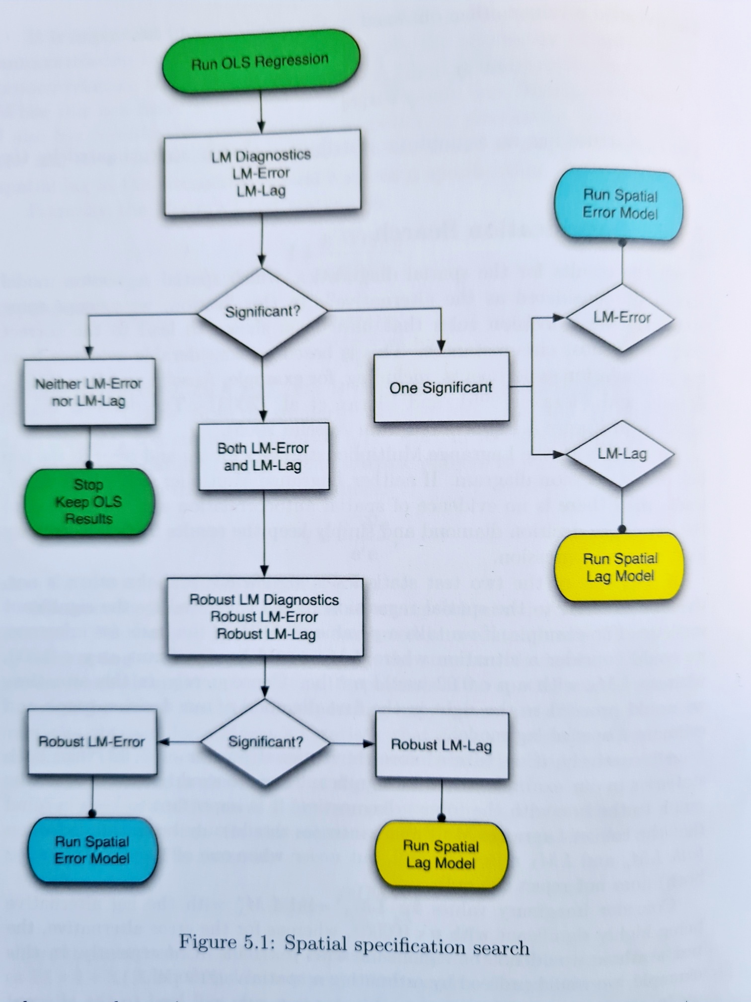<font size = 2>Source: [Modern Spatial Econometrics in Practice](https://www.amazon.co.uk/Modern-Spatial-Econometrics-Practice-GeoDaSpace/dp/0986342106){target="_blank}</font>In the first step, we find that in this instance both the LM-Error and LM-Lag tests are significant.```{r}ols4 <-lm(Rate ~ IMD + age0.11+ age25.34+ age50.59+ carebeds +poly(density, 2), data = covid)lm.LMtests(ols4, spweight, test=c("LMerr", "LMlag"))```Moving on to the robust tests, only the LM-Lag test is significant. Given the nature of COVID-19 as an infectious disease, it does seem reasonable to suppose that high rates of infection in any an area will 'overspill' into neighbouring areas too.```{r}lm.LMtests(ols4, spweight, test=c("RLMerr", "RLMlag"))```## A geographically weighted spatial weights matrixAs with the tests of spatial autocorrelation in an earlier session and as with the geographically weighted statistics, the results of the spatial regression models are dependent on the specification of the spatial weights matrix which can suffer from being somewhat arbitrary. We could, if we wish, try calibrating it around the geographically weighted mean.```{r}#| results: falserequire(GWmodel)bw <-bw.gwr(Rate ~1, data = covid_sp, adaptive =TRUE, kernel ="bisquare")```To now create the corresponding inverse distance spatial weights matrix for the models, we can use the `nn2` function in the `RANN` package to find the $bw = $ `r bw` nearest neighbours to each centroid point:```{r}if(!("RANN"%in%installed.packages()[,1])) install.packages("RANN")require(RANN)coords <-st_coordinates(st_centroid(st_geometry(covid)))knn <-nn2(coords, coords, k = bw)```Having done so, those neighbours can be geographically weighted using a bisquare kernel, as in the GWR calibration above. (A Gaussian kernel is obtained if `(1 - (x / max(x))^2)^2` is replaced by `exp(-0.5 * (x / max(x))^2)` in the code below).```{r}d <- knn$nn.distsglist <-apply(d, 1, \(x) { (1- (x /max(x))^2)^2}, simplify =FALSE)knearnb <-knn2nb(knearneigh(st_centroid(st_geometry(covid)), k = bw))spweightK <-nb2listw(knearnb, glist, style ="C")```The results are not very successful though. The lag model with contiguous spatial weights fits the data better,```{r}lagmod3 <-lagsarlm(formula(ols4), data = covid, listw = spweightK)bind_rows(glance(lagmod2), glance(lagmod3))```In addition, the inverse distance weights are not row-standardised, which may cause some knock-on problems. They could become row-standardised (`spweightK <- nb2listw(knearnb, glist, style = "W")`) but if they are, by re-scaling each row of the weights to equal one, then the inverse distance weighting is altered.## Geographically Weighted RegressionThe following charts shows the simple, bivariate regression relationship between `Rate` and `age0.11`.```{r}#| fig.height = 3ggplot(covid, aes(x = age0.11, y = Rate)) +geom_point() +geom_smooth(method ="lm", se =FALSE)```Intriguingly, it doesn't seem to be linear relationship but a polynomial one.```{r}#| fig.height = 3ggplot(covid, aes(x = age0.11, y = Rate)) +geom_point() +geom_smooth(method ="lm", se =FALSE, formula = y ~poly(x, 2))```It could be that the relationship is indeed curved but it might also be that the nature of the relationship is spatially dependent -- that the relationship between `Rate` and `age0.11` depends upon where it is measured. A `coplot()` from R's base graphics lends weight to the second idea: note how the regression relationship changes with `X` and `Y`, which are the centroids of the neighbourhoods in the North West of England.```{r}#| fig.height = 6coplot_df <-data.frame(st_coordinates(st_centroid(covid)), Rate = covid$Rate, age0.11 = covid$age0.11)PointsWithLine =function(x, y, ...) {points(x=x, y=y, pch=20, col="black")abline(lm(y ~ x))}coplot(Rate ~ age0.11| X * Y, data = coplot_df, panel = PointsWithLine, overlap =0)```Imagine, now, that instead of dividing the geography of the North West's neighbourhoods into a $6 \times 6$ grid, as in the coplot, we instead go from location to location within the study region, calculating a [geographically weighted regression](https://www.sciencedirect.com/science/article/pii/B9780080449104004478?via%3Dihub){target="_blank"} at and around each one of them. This builds on the idea of geographically weighted statistics that allow the measured value of the statistic to vary locally from location to location across the study region; with geographically weighted it is the locally estimated regression coefficients that are allowed to vary. These are used to look for spatial variation in the regression relationships.If the bandwidth is not known or there is no theoretical justification for it, it can be found using an automated selection procedure, here with a more complex model than the bivariate relationship shown in the coplot, instead using all the variables included in the choice between the spatial error and lagged y model, above.```{r}#| results: falserequire(GWmodel)bw <-bw.gwr(formula(ols4), data = covid_sp, adaptive =TRUE)```The model can then be fitted.```{r}gwrmod <-gwr.basic(formula(ols4), data = covid_sp, adaptive =TRUE, bw = bw)gwrmod```The output requires some interpretation! The results of the global regression are those obtained from a standard OLS regression (i.e. `summary(lm(formula(ols4), data = covid_sp))`). It is 'global' because it is a model for the entire study region, without spatial variation in the regression estimates. The results of the geographically weighted regression are the results from, in this case, `r nrow(covid)` separate but spatially overlapping regression models fitted, with geographic weighting, to spatial subsets of the data. All the local estimates are contained in the spatial data frame, `gwrmod$SDF`, including those for `age0.11` which are in `gwrmod$SDF$age0.11` and have the following distribution,```{r}summary(gwrmod$SDF$age0.11)```This is the same summary of the distribution that is included in the GWR coefficient estimates. What it means is that in at least one location the relationship of `age0.11` to `Rate` is, conditional on the other variables, negative. It is more usual for it to be positive -- more children, more infections (perhaps a school effect?) -- but the estimated effect size varies quite substantially across the locations in the study region. Its interquartile range is from `r round(quantile(gwrmod$SDF$age0.11, probs = 0.25), 3)` to `r round(quantile(gwrmod$SDF$age0.11, probs = 0.75), 3)`. Mapping these local estimates reveals an interesting geography -- it is largely in and around Manchester where a greater number of children of primary school age or younger appears to *lower* instead of raising the infection rate.```{r}covid$age0.11GWR <- gwrmod$SDF$age0.11ggplot(data = covid, aes(fill = age0.11GWR)) +geom_sf(size =0.25) +scale_fill_gradient2("beta", mid ="grey90", trans ="reverse") +theme_void() +guides(fill =guide_colourbar(reverse =TRUE))```With a bit of effort we can get all the variables on the same chart...```{r}if(!("gridExtra"%in%installed.packages()[,1])) install.packages("gridExtra",dependencies =TRUE)require(gridExtra)g <-lapply(2:8, \(j) {st_as_sf(gwrmod$SDF[, j]) %>%rename(beta =1) %>%ggplot(aes(fill = beta)) +geom_sf(col =NA) +scale_fill_gradient2("beta", mid ="grey90", trans ="reverse") +theme_void() +guides(fill =guide_colourbar(reverse =TRUE)) +ggtitle(names(gwrmod$SDF[j]))})grid.arrange(grobs = g)```... however, not all of these regression estimates are necessarily statistically significant. If we use the estimated t-values to isolate those that are not (t-values less than -1.96 or greater than +1.96 can be considered significant at a 95% confidence), then, for the `age0.11` variable we obtain,```{r}covid$age0.11GWR[abs(gwrmod$SDF$age0.11_TV) <1.96] <-NAggplot(data = covid, aes(fill = age0.11GWR)) +geom_sf(size =0.25) +scale_fill_gradient2("beta", mid ="grey90", na.value ="white",trans ="reverse") +theme_void() +guides(fill =guide_colourbar(reverse =TRUE))```and, with a bit more data wrangling, for the full set,```{r}sdf <-slot(gwrmod$SDF, "data")g <-lapply(2:8, \(j) { x <-st_as_sf(gwrmod$SDF[, j]) t <-which(names(sdf) ==paste0(names(x)[1],"_TV")) x[abs(sdf[, t]) <1.96, 1] <-NA x %>%rename(beta =1) %>%ggplot(aes(fill = beta)) +geom_sf(col =NA) +scale_fill_gradient2("beta", mid ="grey90", na.value ="white",trans ="reverse") +theme_void() +guides(fill =guide_colourbar(reverse =TRUE)) +ggtitle(names(gwrmod$SDF[j]))})grid.arrange(grobs = g)```{width=75}<font size = 3>I am sure there is a more elegant way of doing this. Don't worry about the code especially - the point is that not every estimate, everywhere, is significant.</font></br>As with the basic GW statistics, we can undertake a randomisation test to suggest whether the spatial variation in the coefficient estimates is statistically significant. **However** this takes some time to run -- with the default `nsims = 99` simulations it took about 12 minutes on my laptop. **I have 'commented it out' in the code block below with the suggestion that you don't run it now.**```{r}# I suggest you do not run this# gwr.mc <- gwr.montecarlo(formula(ols4), covid_sp, adaptive = TRUE, bw = bw)```Instead, let's jump straight to the results, which I have saved in a pre-prepared workspace.```{r}url <-url("https://github.com/profrichharris/profrichharris.github.io/raw/main/MandM/workspaces/gwrmc.RData")load(url)close(url)gwr.mc```### Mixed GWR**I suggest you just read over this section rather than do it because it takes some time to run**It appears that only the `age0.11` and `density` variables exhibit significant spatial variation (p-value < 0.05). In principle it is possible to drop the other variables out from the local estimates and treat them as fixed, global estimates instead, in a Mixed GWR model (mixed global and local regression estimates). In the past it has generated an error for me but maybe it will work now?```{r}#| eval: false# This appears to generate an errorgwrmixd <-gwr.mixed(Rate ~ IMD + age0.11+ age25.34+ age50.59+ carebeds +poly(density, 2),data = covid_sp,fixed.vars =c("IMD", "age25.34", "age50.59", "carebeds"),bw = bw, adaptive =TRUE)```If it does not work, We can work around it, using partial regressions, regressing `Rate`, `age0.11` and `poly(density, 2)` on the fixed variables and using their residuals.```{r}#| eval: falsedensity.1<-poly(covid$density, 2)[, 1]density.2<-poly(covid$density, 2)[, 2]covid_sp$RateR <-residuals(lm(Rate ~ IMD + age25.34+ age50.59+ carebeds,data = covid_sp))covid_sp$age0.11R <-residuals(lm(age0.11~ IMD + age25.34+ age50.59+ carebeds, data = covid_sp))covid_sp$density.1R <-residuals(lm(density.1~ IMD + age25.34+ age50.59+ carebeds, data = covid_sp))covid_sp$density.2R <-residuals(lm(density.2~ IMD + age25.34+ age50.59+ carebeds, data = covid_sp))fml <-formula(RateR ~ age0.11R + density.1R + density.2R)bw <-bw.gwr(fml, data = covid_sp, adaptive =TRUE)gwrmixd <-gwr.basic(fml, data = covid_sp, bw = bw, adaptive =TRUE)```The following code block with them highlight the statistically significant results for the `age0.11` variable.```{r}#| eval: falsecovid$age0.11GWR <- gwrmixd$SDF$age0.11Rcovid$age0.11GWR[abs(gwrmixd$SDF$age0.11R_TV) >1.96] <-NAggplot(data = covid, aes(fill = age0.11GWR)) +geom_sf(size =0.25) +scale_fill_gradient2("beta", mid ="grey90", na.value ="white", trans ="reverse") +theme_void() +guides(fill =guide_colourbar(reverse =TRUE))```### Multiscale GWRIt is also possible to fit a Multiscale GWR, which allows for the possibility of a different bandwith for each variable -- see `?gwr.multiscale`. Since there is no particular reason to presume that the bandwidth should be the same for all the variables, arguably Multiscale GWR should be preferred over standard GWR, at least in the first instance. Its main drawback, however, is that it takes a while to run -- over 3 hours for the code chunk below! (In principle it can be parallelised but it generated an error for me when I tried this with `parallel.method = cluster`.)```{r}#| eval: falsedensity.1<-poly(covid$density, 2)[, 1]density.2<-poly(covid$density, 2)[, 2]# Do not run!# Took over 3 hours!#gwrmulti <- gwr.multiscale(Rate ~ IMD + age0.11 + age25.34 + age50.59 + carebeds +# density.1 + density.2, data = covid_sp, adaptive = TRUE)```To save time, the results are available below. The bandwidths do appear to vary.```{r}url <-url("https://github.com/profrichharris/profrichharris.github.io/raw/main/MandM/workspaces/gwrmulti.RData")load(url)close(url)gwrmulti```### Geographically and temporally weighted regressionIt also possible to add a time dimension and undertake geographically and temporally weighted regression in `GWmodel`. The following workspace loads monthly COVID-19 data for Manchester neighbourhoods.```{r}url <-url("https://github.com/profrichharris/profrichharris.github.io/raw/main/MandM/workspaces/manchester.RData")load(url)close(url)```Here are the monthly rates.```{r}ggplot(covid, aes(fill = Rate )) +geom_sf() +facet_wrap(~ month) +scale_fill_distiller(palette ="RdBu") +theme_void()```If now want to explore how the regression relationships vary in space-time then we can use the `bw.gtwr()` and `gtwr()` functions, for which we also need to specify a vector of time tags (`obs.tv = ...`). In these data, they are simply a numeric value, `covid$month_code` but see `?bw.gtwr()` and `?gtwr()` for further possibilities and for further information about the model.{width=75}<font size = 3>The model will take a little time to run -- enough time for you to get a cup of tea or coffee!</font>```{r}#| eval: falsecovid_sp <-as_Spatial(covid)fml <-formula(Rate ~ IMD + age0.11+ age25.34+ age50.59+ carebeds +poly(density, 2))bw <-bw.gtwr(fml, data = covid_sp, obs.tv = covid$month_code, adaptive =TRUE)gtwrmod <-gtwr(fml, data = covid_sp, st.bw = bw, obs.tv = covid$month_code, adaptive =TRUE)``````{r}#| include: falseurl <-url("https://github.com/profrichharris/profrichharris.github.io/raw/main/MandM/workspaces/gtwrmod.RData")load(url)close(url)```Here are the summary results of the model,```{r}gtwrmod```They should be treated cautiously because the `Rate` value is strongly positively skewed such that it may have been better to have transformed it (e.g. taken its square root) prior to analysis. Even so, there is some evidence that the predictor `age0.11` variable, for example, varies spatially *and* temporally.```{r}covid$age0.11GWR <- gtwrmod$SDF$age0.11covid$age0.11GWR[abs(gtwrmod$SDF$age0.11_TV) <1.96] <-NAggplot(covid, aes(fill = age0.11GWR)) +geom_sf() +facet_wrap(~ month) +scale_fill_gradient2("beta", mid ="grey90", na.value ="white", trans ="reverse") +theme_void() +guides(fill =guide_colourbar(reverse =TRUE))```### Generalised GWR models with Poisson and Binomial optionsSee `?ggwr.basic`.## SummaryIn this session we have looked at spatial regression models as a way to address the problem of spatial autocorrelation in regression residuals and to allow for the possibility that regression relationships vary across a map. In presenting these methods, at least some could be taken as offering a 'technical fix' to the statistical issue of spatial dependencies in the data, violating assumptions of independence. Whilst that may be true, and the more spatial approaches can be used as diagnostic tools to check for a mis-specified model, notably one that lacks a critical explanatory variable or where the relationship between the X and Y variables is non-linear, the limitation of this thinking is that it treats geography as an error to be resolved and/or it rests on the belief that with sufficient information the geographical differences will be explained. What geographically weighted regression, for example, reminds us is that the nature of the relationship may be complex because it is changing in form across the study region as the socio-spatial causes also vary from place to place. Such spatial complexity may be challenging to accommodate within the parameters of conventional aspatial or spatially naïve statistical thinking but ignoring the geographical variation is not a solution. What spatial thinking brings to the table is the recognition of geographical context and the knowledge that geographically rooted social outcomes are not independent of where the processes giving rise to those outcomes are taking place. ## Further Reading{width=100}[Spatial Regression Models (2nd edition) by MD Ward & KS Gleditsch (2018)](https://uk.sagepub.com/en-gb/eur/spatial-regression-models/book262155){target="_blank"}Comber et al. (2022) A Route Map for Successful Applications of Geographically Weighted Regression. [https://doi.org/10.1111/gean.12316](https://doi.org/10.1111/gean.12316){target="_blank"}