There are lots of ways to produce maps in R. But, however, they are drawn, two things are usually needed to produce a choropleth map of the sort seen in previous sessions:
first, some data;
second, a map to join the data to.
The join is usually made possible by the data and the map containing the same variable; for example, by using the same ID codes for all the places in the data as are in the map. This implies that what is contained in the data set are measurements of the places shown in the map. Sometimes maps will come pre-bundled with the data of interest so, in effect, the join has already been made.
Once we have the data ready to map (sometimes by ‘cleaning’ the data before linking them to the map) then R offers plenty of options to produce quick or publication quality maps, which may have either static or dynamic content. The two packages we shall focus on are:
Another package we shall be using in this session is sf, which provides “support for simple features, a standardized way to encode spatial vector data.” What we are mapping in this exercise are vector data – data for which the geography is ultimately defined by a series of points (two points define a line, a series of lines define a boundary, a boundary demarcates an area, and so forth). The other common geographic representation used in Geographic Information Systems is raster, which is a grid representation of a study region, with each cell in the grid given one or more values to represent what is found there. For raster data, the stars and raster packages are useful.
Part 1
Getting Started
As in previous sessions, if you are keeping all the files and outputs from these exercises together in an R Project (which is a good idea) then open that Project now.
Load the data
Let’s begin with the easy bit and load the data, which are from http://superweb.statssa.gov.za. These includes the variable No_schooling which is the percentage of the population without schooling per South African municipality in 2011.
Code
# A quick check to see if the Tidyverse packages are installed...installed <-installed.packages()[,1]if(!("tidyverse"%in% installed)) install.packages("tidyverse",dependencies =TRUE)require(tidyverse)# Read-in the data directly from a web location. The data are in .csv formateducation <-read_csv("https://github.com/profrichharris/profrichharris.github.io/raw/main/MandM/data/education.csv")# Quick check of the data by looking at the top three rowsslice_head(education, n =3)
We have the data but now we need a ‘blank map’ of the same South African municipalities to map it. It is read-in below in geoJSON format but it would not have been unusual if it had been in .shp (shapefile) or .kml format, instead. The source of the data is https://dataportal-mdb-sa.opendata.arcgis.com/. There are several ways of reading this file into R but it is better to use the sf package because older options such as maptools::readShapePoly() (which was for reading shapefiles) or rgdal::readOGR are either deprecated already or in the process of being retired.
Code
# Another quick check to make sure that various libraries have been installedif(!("proxy"%in% installed)) install.packages("proxy")if(!("sf"%in% installed)) install.packages("sf", dependencies =TRUE)require(sf)# Use the read_sf() function from the sf library to read in a digital map of the study areamunicipal <-read_sf("https://github.com/profrichharris/profrichharris.github.io/raw/main/MandM/boundary%20files/MDB_Local_Municipal_Boundary_2011.geojson")
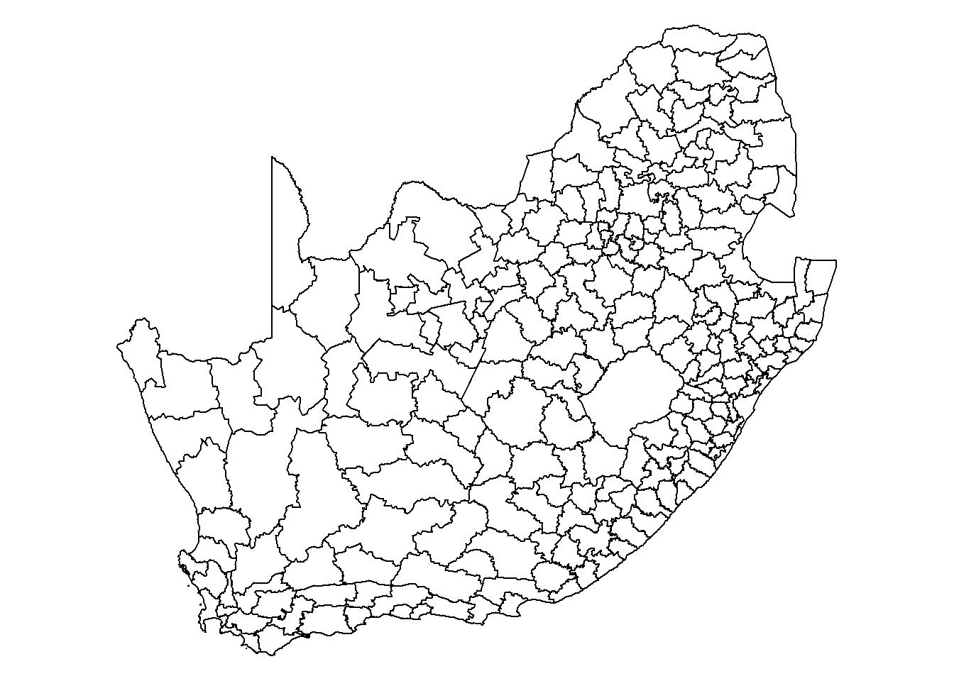
If we now look at the top of the municipal object then we find it is of class sf, which is short for simple features. It has a vector geometry (it is of type multipolygon) and has its coordinate reference system (CRS) set as WGS 84. It also contains some attribute data, although not the schooling data we are looking to map.
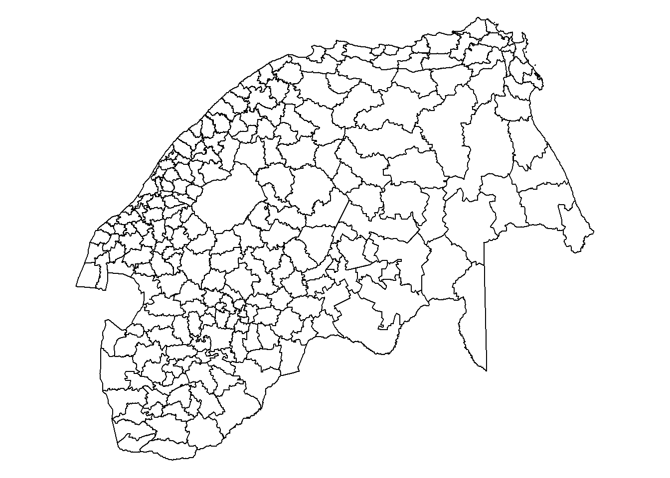
Had it been necessary to set the coordinate reference system (CRS) then the function st_set_crs() would be used. Instead, and just for fun, we will change the existing CRS: here is the map transformed on to a ‘south up’ coordinate reference system, achieved by changing its EPSG code to 2050 with the function st_transform(). I have no idea why you would want to do this or what the projection is actually used for but, more generally, the st_transform is useful for, say (not here, but in other cases), converting between the UK National Grid system (EPSG:27700) and longitude and latitude (EPSG:4326), or making sure the maps you are working with are all using the same CRS, which would be necessary for various GIS (Geographic Information Systems) type operations.
Note how functions with the sf library tend to start with st_. Personally, I find this slightly confusing and I am not sure it makes it easier to find what I looking for in the package’s help pages but it is consistent for the functions and methods that operate on spatial data and is, I believe, short for spatial type.
sf and sp
At the risk of over-simplification, sf (simple features) can be viewed as a successor to the earlier sp (spatial) and related packages, which are well documented in the book Applied Spatial Data Analysis with R. Sometimes other packages are still reliant on sp and so the spatial objects need to be changed into sp’s native format prior to use.
Code
# From sf to spmunicipal_sp <-as(municipal, "Spatial")class(municipal_sp)
# From sp to sfmunicipal_sf <-st_as_sf(municipal_sp)class(municipal_sf)
[1] "sf" "data.frame"
The need for this ought to be less frequent now that sf is well established and sp deprecated.
Joining the attribute data to the map
If we look again at the map and schooling data, we find that they have two variables in common which suggests a means to join them together based on a common variable.
Code
# The variables that they appear to have in common...intersect(names(municipal), names(education))
This is encouraging but, in this example, we need to be careful using the municipal names because not all of those in the map are in the education data or vice versa. Although the variable LocalMunicipalityName is present in both the map and education data, the variable is not actually the same in both because of different ways of spelling the names of places. The following code shows where one is not the same as the other.
Code
# anti_join() returns all rows from x without a match in yanti_join(municipal, education, by ="LocalMunicipalityName")
Simple feature collection with 7 features and 10 fields
Geometry type: MULTIPOLYGON
Dimension:     XY
Bounding box:  xmin: 27.42423 ymin: -32.05935 xmax: 32.05014 ymax: -24.96652
Geodetic CRS:  WGS 84
# A tibble: 7 × 11
  OBJECTID ProvinceCode ProvinceName LocalMunicipalityCode LocalMunicipalityName
     <int> <chr>        <chr>        <chr>                 <chr>
1       34 EC           Eastern Cape EC157                 King Sabata Dalindye
2       74 KZN          KwaZulu-Nat… KZN214                uMuziwabantu
3       75 KZN          KwaZulu-Nat… KZN215                Ezinqoleni
4       97 KZN          KwaZulu-Nat… KZN262                uPhongolo
5      146 MP           Mpumalanga   MP301                 Chief Albert Luthuli
6      149 MP           Mpumalanga   MP304                 Dr Pixley Ka Isaka S
7      165 NW           North West   NW372                 Local Municipality o
# ℹ 6 more variables: DistrictMunicipalityCode <chr>,
#   DistrictMunicipalityName <chr>, Year <int>, Shape__Area <dbl>,
#   Shape__Length <dbl>, geometry <MULTIPOLYGON [°]>
Code
anti_join(education, municipal, by ="LocalMunicipalityName")
Fortunately, the municipal codes are consistent even where the names are not, which is why place codes and IDs are generally better than using names when joining data. Names are often subject to sometimes subtle variations that can upset the intended join.
Code
# The municipality codes are consistent in the map and data; there are none that do not match.anti_join(municipal, education, by ="LocalMunicipalityCode")
Simple feature collection with 0 features and 10 fields
Bounding box:  xmin: NA ymin: NA xmax: NA ymax: NA
Geodetic CRS:  WGS 84
# A tibble: 0 × 11
# ℹ 11 variables: OBJECTID <int>, ProvinceCode <chr>, ProvinceName <chr>,
#   LocalMunicipalityCode <chr>, LocalMunicipalityName <chr>,
#   DistrictMunicipalityCode <chr>, DistrictMunicipalityName <chr>, Year <int>,
#   Shape__Area <dbl>, Shape__Length <dbl>, geometry <GEOMETRY [°]>
Code
anti_join(education, municipal, by ="LocalMunicipalityCode")
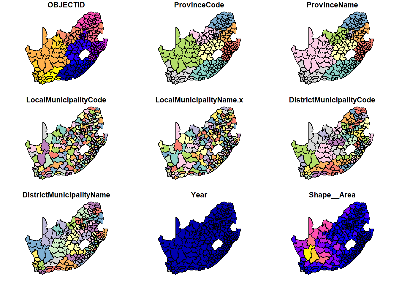
Note that the variables LocalMunicipalityName.x and LocalMunicipalityName.y have been created in the process of the join. This is because although we did not use LocalMunicipalityName for the join, that variable name is present in both the map and the data and is therefore duplicated when they are joined together – municipal$LocalMunicipalityName becomes municipal$LocalMunicipalityName.x and education$LocalMunicipalityName creates municipal$LocalMunicipalityName.y.
Mapping the data
Using plot{sf}
The ‘one line’ way of plotting the data is to use the in-built plot() function for sf.
Code
plot(municipal["No_schooling"])
As a ‘rough and ready’ way to check for spatial variation and patterns in the data, it is quick and easy. It is important to specify the variable(s) you wish to include in the plot – plot(municipal["No_schooling"]) in the example above – or else it will try and plot all of them in the map’s data, up to the value specified by the argument max.plot, which has a default of nine.
Code
plot(municipal)
The map can be customised. For example,
Code
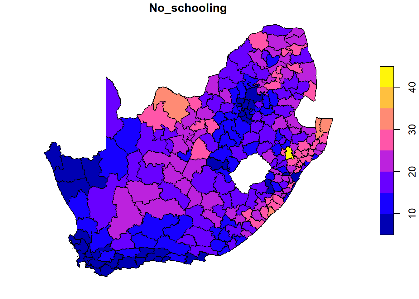
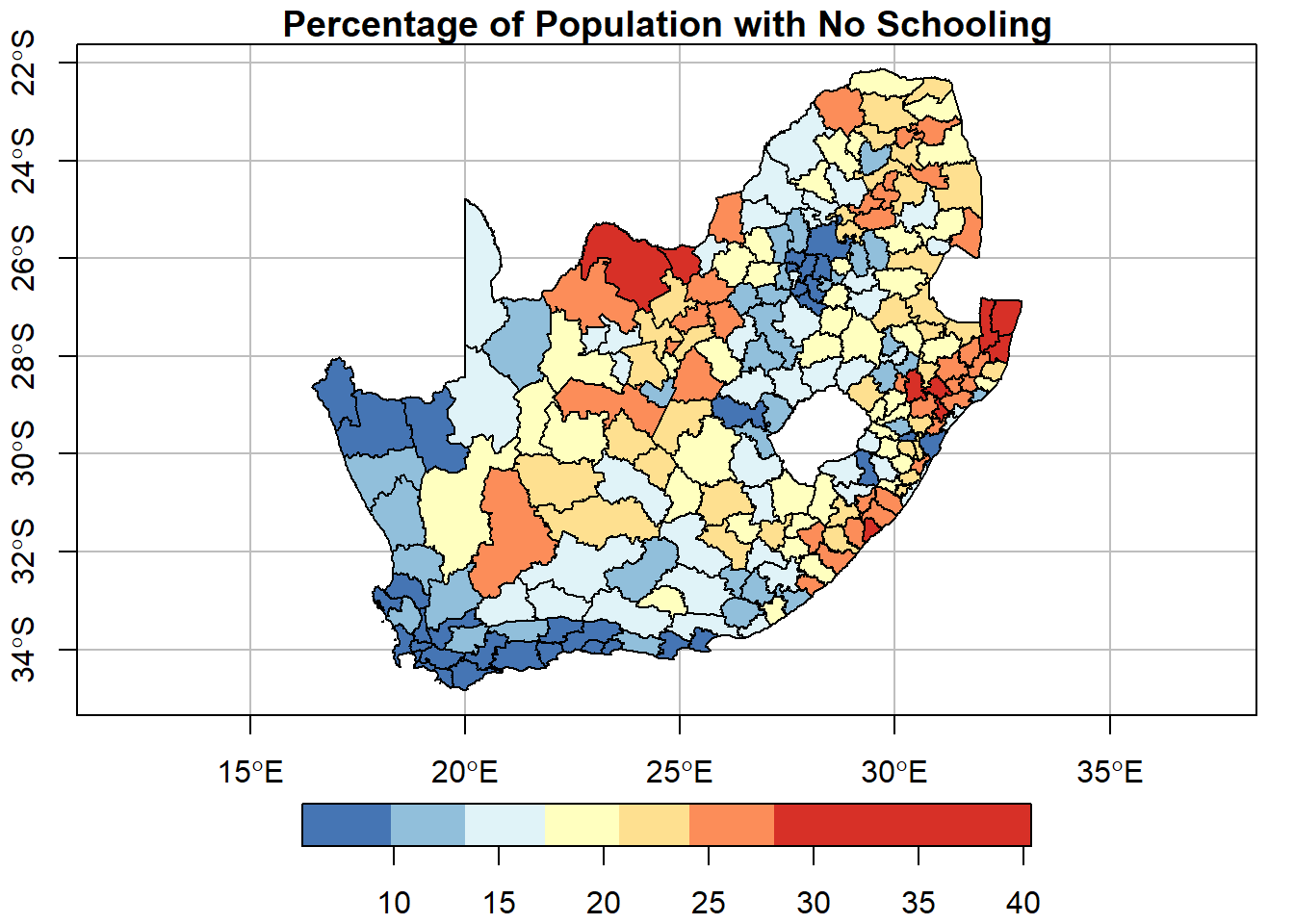
if(!("RColorBrewer"%in% installed)) install.packages("RColorBrewer",dependencies =TRUE)require(RColorBrewer)plot(municipal["No_schooling"], key.pos =1, breaks ="jenks", nbreaks =7,pal =rev(brewer.pal(7, "RdYlBu")),graticule =TRUE, axes =TRUE,main ="Percentage of Population with No Schooling")
Have a read through the documentation at ?sf::plot to get a sense of what the various arguments do. Try changing them and see if you can produce a map with six equal interval breaks, for example.
Note the use of the RColorBrewer package and its brewer.pal() function. RColorBrewer provides colour palettes based on https://colorbrewer2.org/ and has been used to create a diverging red-yellow-blue colour palette that is reversed using the function rev() so that red is assigned to the highest values, not lowest. A ‘natural breaks’ (jenks) classification with 7 colours has been used (breaks = "jenks", nbreaks = 7).
Thinking about the map classes
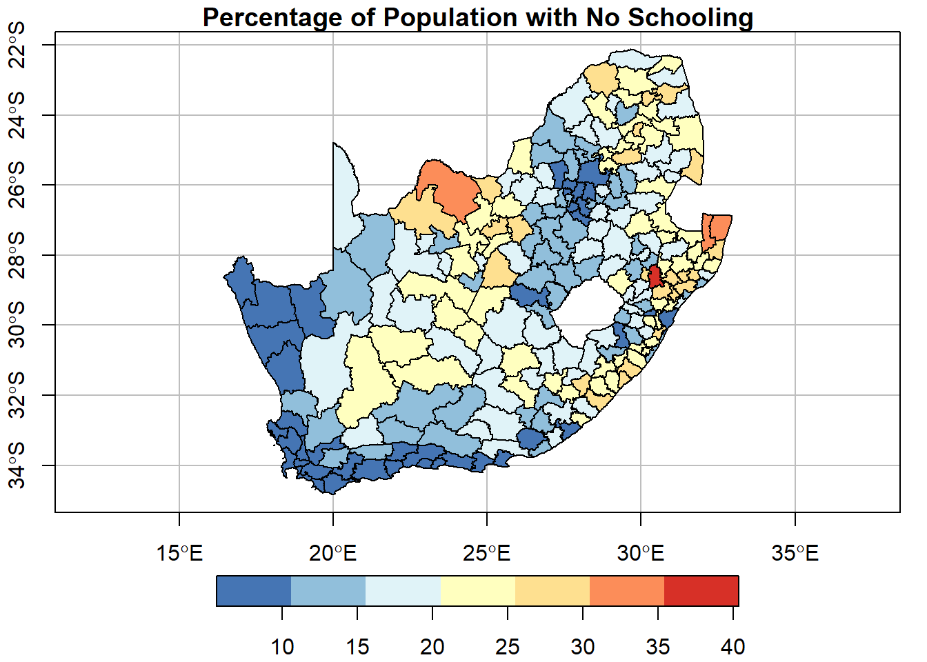
It is obvious, but under-appreciated, that what we see in a map in a function of how the map is constructed, including the map classes used. Here is the same underlying map but with equal interval breaks instead:
Code
plot(municipal["No_schooling"], key.pos =1, breaks ="equal", nbreaks =7,pal =rev(brewer.pal(7, "RdYlBu")),graticule =TRUE, axes =TRUE,main ="Percentage of Population with No Schooling")
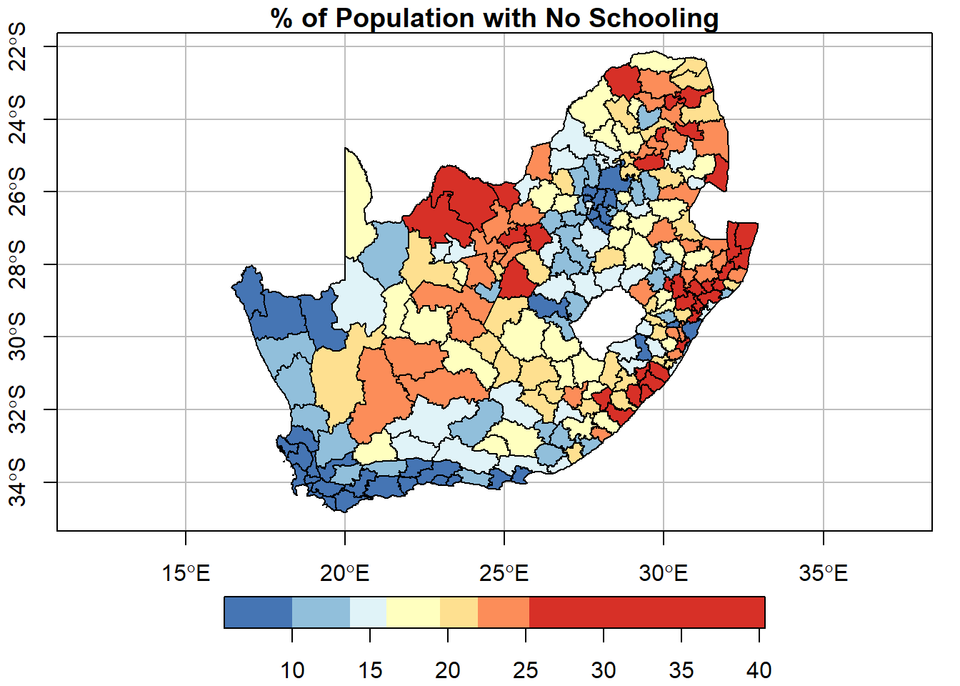
… and here it is with quantile breaks:
Code
plot(municipal["No_schooling"], key.pos =1, breaks ="quantile", nbreaks =7,pal =rev(brewer.pal(7, "RdYlBu")),graticule =TRUE, axes =TRUE,main ="% of Population with No Schooling")
Clearly the maps above do not appear exactly the same. The geographical patterns and therefore the geographical information that we view in the map change with the number, colouring and widths (ranges) of the map classes. Ideally, these should be set to reflect the distribution of the data and what is being look for in it.
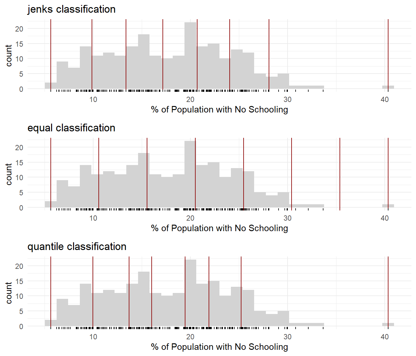
Let’s explore that distribution for a moment and how the various map classes used above end up dividing it up. The following histograms show the break points in the distributions used in the various maps. The code works by creating a list of plots (specifically, a list of ggplots, see below) – one plot each for the jenks, equal and quantile styles – and then, using a package called gridExtra, to arrange those plots into a single grid. However, the code matters less than what it reveals, which is that Jenks or other ‘natural breaks’ classifications are reasonably good for identifying break points that reflect the distribution of the data in the absence of the user having cause to set those break points in some other way.
I am not suggesting you need to follow these exact steps every time you want to map but some data. BUT thinking about the distribution of the data is always important to avoid creating maps that give the wrong impression of the prevalence or otherwise of values in the data. For example, if you use a quantile classification with, say, 4 breaks, it will create four map classes, each containing approximately one quarter of the data, even if some of the values in those classes are rarely found and are unusual when compared to others in the same class. An equal interval classification will not have this problem.
Code
if(!("gridExtra"%in% installed)) install.packages("gridExtra",dependencies =TRUE)if(!("classInt"%in% installed)) install.packages("classInt",dependencies =TRUE)require(gridExtra)require(classInt)styles <-c("jenks", "equal", "quantile")g <-lapply(styles, \(x) {ggplot(municipal, aes(x = No_schooling)) +geom_histogram(fill ="light grey") +xlab("% of Population with No Schooling") +geom_vline(xintercept =classIntervals(municipal$No_schooling,n =7, style = x)$brks,col ="dark red") +geom_rug() +theme_minimal() +ggtitle(paste(x,"classification")) })# The step below brings together, in a grid, the list of three different plots# created abovegrid.arrange(grobs = g)
For further information on using plot{sf} see here and look at the help menu, ?sf::plot.
Using ggplot2
Whilst the plot() function for sf objects is useful for producing quick maps, I prefer ggplot2 for better quality ones that I am wanting to customise or annotate in particular ways, or to include in a research publication or report. We already have seen examples of ggplot2 output in earlier sessions and also in the histograms above.
ggplot2 is based on The Grammar of Graphics. It’s a simplification of the ‘grammar’ but I find it easiest to think of it, initially, in four stages:
Say which data are to be plotted;
Say which aesthetics of the chart (e.g. colour, line type, point size) will vary with the data (or just be constant);
Say which types of plots (which ‘geoms’) are to feature in the chart;
(Optional customisation) change other attributes of the chart to add titles, rename the axis labels, and so forth.
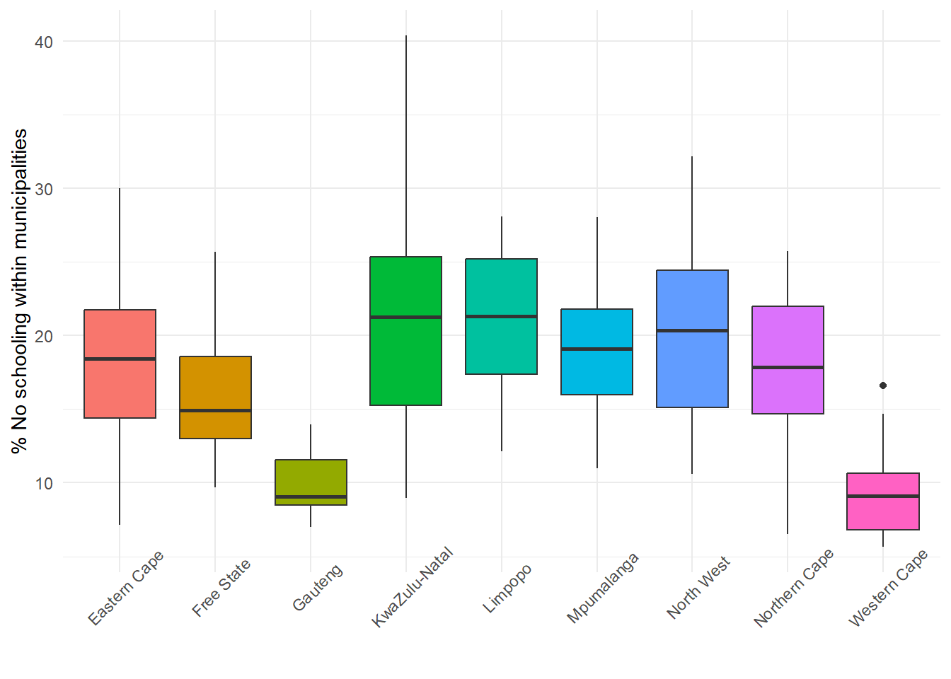
As an example, and in the code chunk below, those four stages are applied to a boxplot showing the distribution of the no schooling variable by South African Provinces.
First, the data = municipal. Second, consulting with the ggplot2 cheatsheet, I find that the aesthetics, aes(), for the boxplot, require a discrete x and a continuous y, which are provided by ProvinceName and No_schooling, respectively. ProvinceName has also been used to assign a fill colour to each box. Third, the optional changes arise from me preferring theme_minimal() to the default style, although I have then modified it to remove the legend, change the angle of the text on the x-axis, remove the x-axis label and change the y-axis label. I did not have to do any of this; I just preferred it.
Code
require(ggplot2)ggplot(data = municipal, aes(x = ProvinceName, y = No_schooling,fill = ProvinceName)) +geom_boxplot() +theme_minimal() +theme(legend.position ="none", axis.text.x =element_text(angle =45)) +xlab(element_blank()) +ylab("% No schooling within municipalities")
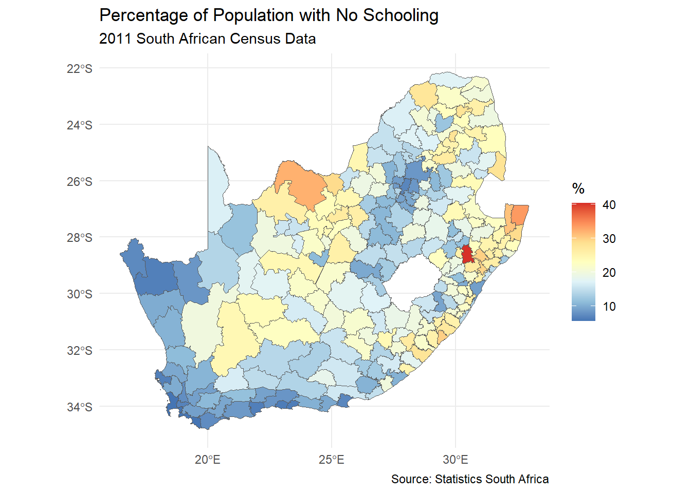
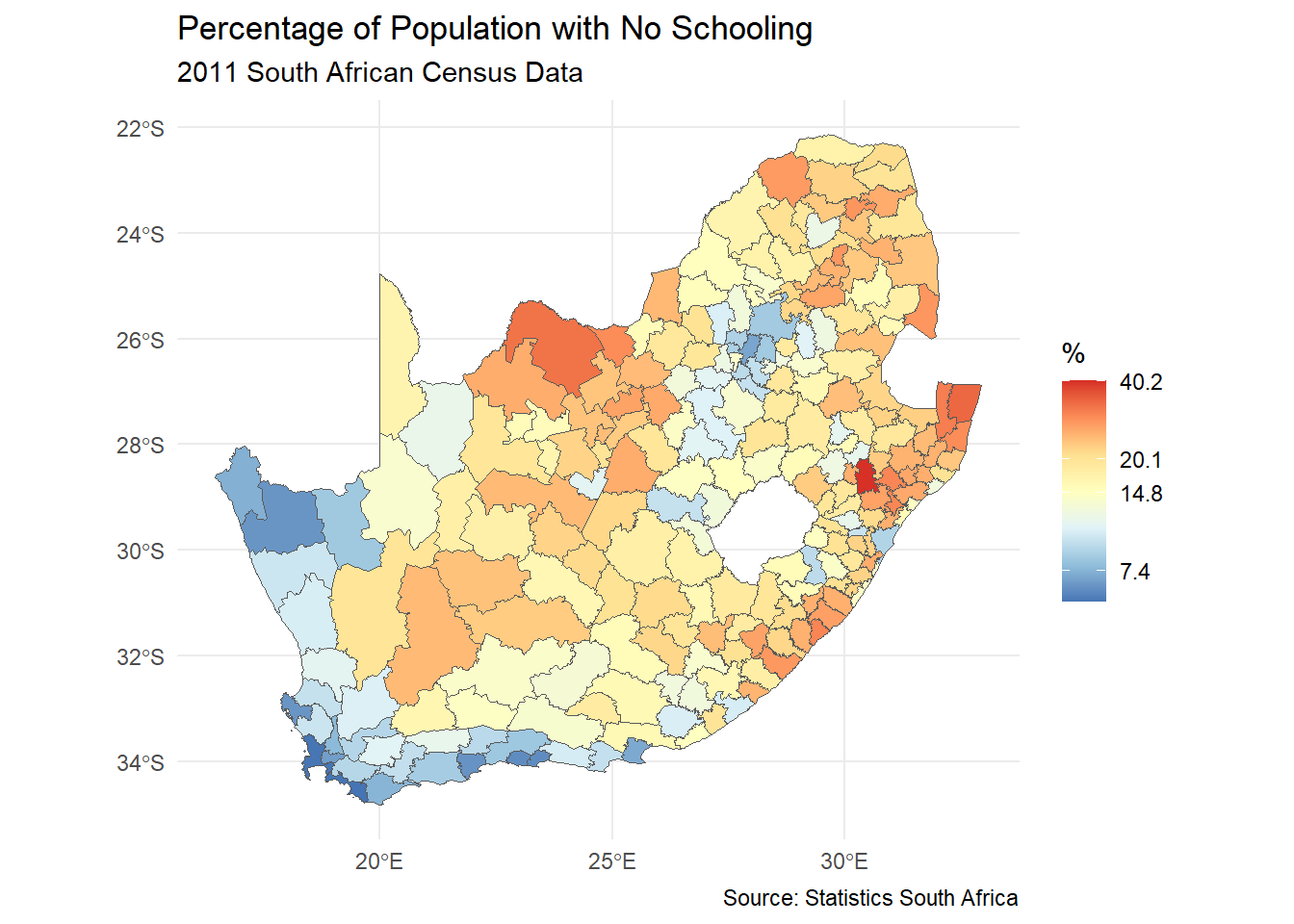
Let’s now take that same general process and apply it to create a map, using the same RColorBrewer colour palette as previously and adding the map using geom_sf (for a full list of geoms available for ggplot2 see here). The line scale_fill_distiller is an easy way to shade the map using the colour palette from RColorBrewer andlabs() adds labelling. The steps are the same: specify the data; specify the aesthetics; specify the geom (now of type sf, because it is a spatial feature); add the customisation.
Code
ggplot(municipal, aes(fill = No_schooling)) +geom_sf() +scale_fill_distiller("%", palette ="RdYlBu") +theme_minimal() +labs(title ="Percentage of Population with No Schooling",subtitle ="2011 South African Census Data",caption ="Source: Statistics South Africa" )
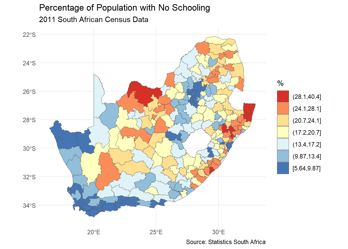
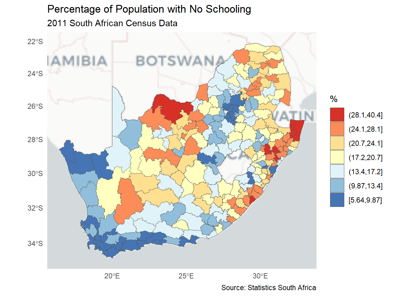
Presently the map has a continuous shading scheme – you can see it in the map’s legend. This can be changed to discrete map classes and colours by converting the continuous municipal$No_schooling variable to a factor, using the cut() function, here with break points found using ClassIntervals(style = "jenks"). Because we have then changed from continuous to discrete (categorised) data but still want to use an RColorBrewer palette, so scale_fill_brewer() replaces scale_fill_distiller(), wherein the argument direction = -1 reverses the RdYlBu palette so that the highest values are coloured red. Adding guides(fill = guide_legend(reverse = TRUE)) reverses the legend so that the highest values are on top in the legend, which is another preference of mine. It just seems kind of logical to me to have the highest values highest in the legend.
Code
# Find the break points in the distribution using a Jenks classificationbrks <-classIntervals(municipal$No_schooling, n =7, style ="jenks")$brks# Factor the No_schooling variable using those break pointsmunicipal$No_schooling_gp <-cut(municipal$No_schooling, brks,include.lowest =TRUE)ggplot(municipal, aes(fill = No_schooling_gp)) +geom_sf() +scale_fill_brewer("%", palette ="RdYlBu", direction =-1) +theme_minimal() +guides(fill =guide_legend(reverse =TRUE)) +labs(title ="Percentage of Population with No Schooling",subtitle ="2011 South African Census Data",caption ="Source: Statistics South Africa" )
At this point, we may note that the four stages of the map production that I referred to earlier was an over-simplification and we can add a fifth (but it is the fourth below; sorry to be confusing):
Say which data are to be plotted;
Say which aesthetics of the chart (e.g. colour, line type, point size) will vary with the data;
Say which types of plots (which ‘geoms’) are to feature in the chart – geom_sf for mapping;
(the new one) ‘Scale’ the data – in the above examples, link the mapped variables to map classes and colour codes. The scaling is what scale_fill_... was doing;
(Optional customisation) change other attributes of the chart to add titles, rename the axis labels, and so forth.
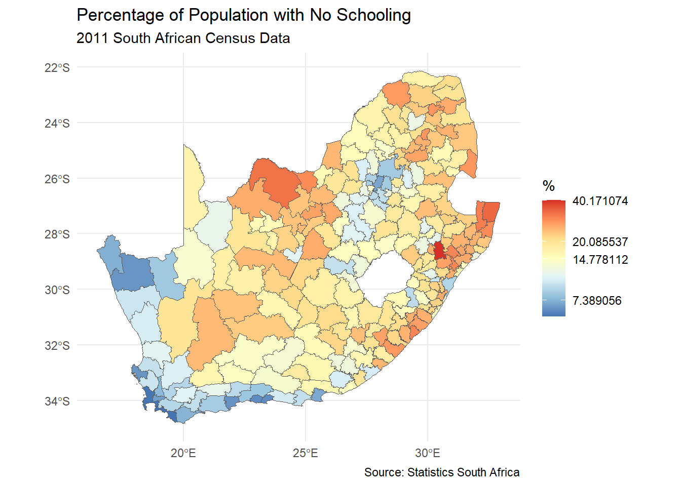
We could also use the scaling to more literally scale (or transform) the data, in a mathematical sense, by using a log scale to plot the data. This will require the original data, before we converted it to factors:
Code
ggplot(municipal, aes(fill = No_schooling)) +geom_sf() +scale_fill_distiller("%", palette ="RdYlBu", trans ="log") +theme_minimal() +labs(title ="Percentage of Population with No Schooling",subtitle ="2011 South African Census Data",caption ="Source: Statistics South Africa" )
The legend of that map would look nicer with the values formatted to a more sensible number of decimal places:
Code
ggplot(municipal, aes(fill = No_schooling)) +geom_sf() +scale_fill_distiller("%", palette ="RdYlBu", trans ="log", label = \(x) sprintf("%.1f", x)) +theme_minimal() +labs(title ="Percentage of Population with No Schooling",subtitle ="2011 South African Census Data",caption ="Source: Statistics South Africa" )
Annotating the map with ggspatial
Having created the basic map using ggplot2, we can add some additional map elements using ggspatial – a package that provides some extra cartographic functions. The following code chunk adds a backdrop to the map. Different backgrounds (alternative map tiles) can be chosen from the list at rosm::osm.types(); see here for what they look like.
Before running the code, we may note a change from the previous code chunk (above) which is in addition to installing and requiring ggspatial and adding the map tile as a backdrop. Specifically, if you look at the previous code chunk you will find that the data, municipal are handed to ggplot in the top line, ggplot(municipal, ...), where the first argument is the data one. In other words, ggplot(municipal, ...) is the same as, ggplot(data = municipal, ...) (check the help file, ?ggplot2::ggplot to confirm this). By specifying the data in the top line, in essence this sets data = municipal as a global parameter for the plot: it is where ggplot will, by default, now look for the variable called for in aes(fill = No_schooling_gp) and where it will look for other variables too. Whilst this would work just fine in the code immediately below, a little later I introduce a second geom_sf into the plot and no longer want municipal to be the default choice for all the aesthetics of the chart, just some of them. To pre-empt any problems that might otherwise arise, I no longer specify municipal as the default dataset in my ggplot() but, instead, specifically name municipal where I want to use it, which is as the fill data, in the line geom_sf(data = municipal, aes(fill = No_schooling_gp)). This will leave me free to associate other data with different aesthetics in due course. More simply, if you set the data = argument and also any aesthetics, mapping = aes() in the ggplot(...) line of the code, then you are basically saying “use these for everything that follows” unless you override them by saying what you want for each specific geom.
Code
if(!("ggspatial"%in% installed)) install.packages("ggspatial",dependencies =TRUE)require(ggspatial)ggplot() +annotation_map_tile(type ="cartolight", progress ="none") +geom_sf(data = municipal, aes(fill = No_schooling_gp)) +scale_fill_brewer("%", palette ="RdYlBu", direction =-1) +theme_minimal() +guides(fill =guide_legend(reverse =TRUE)) +labs(title ="Percentage of Population with No Schooling",subtitle ="2011 South African Census Data",caption ="Source: Statistics South Africa" )
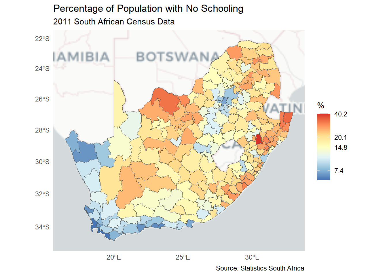
Or, using our previous log scale,
Code
ggplot() +annotation_map_tile(type ="cartolight", progress ="none") +geom_sf(data = municipal, aes(fill = No_schooling)) +scale_fill_distiller("%", palette ="RdYlBu", trans ="log", label = \(x) sprintf("%.1f", x)) +theme_minimal() +labs(title ="Percentage of Population with No Schooling",subtitle ="2011 South African Census Data",caption ="Source: Statistics South Africa" )
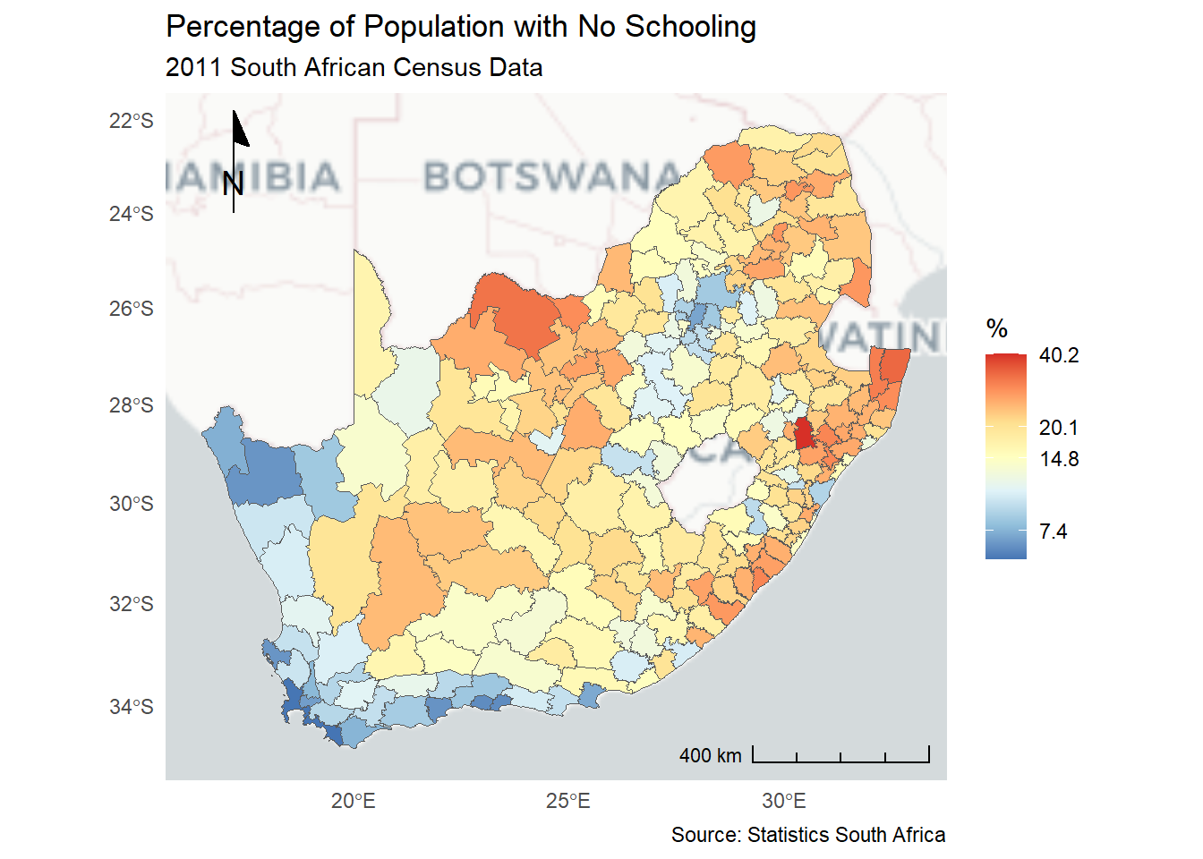
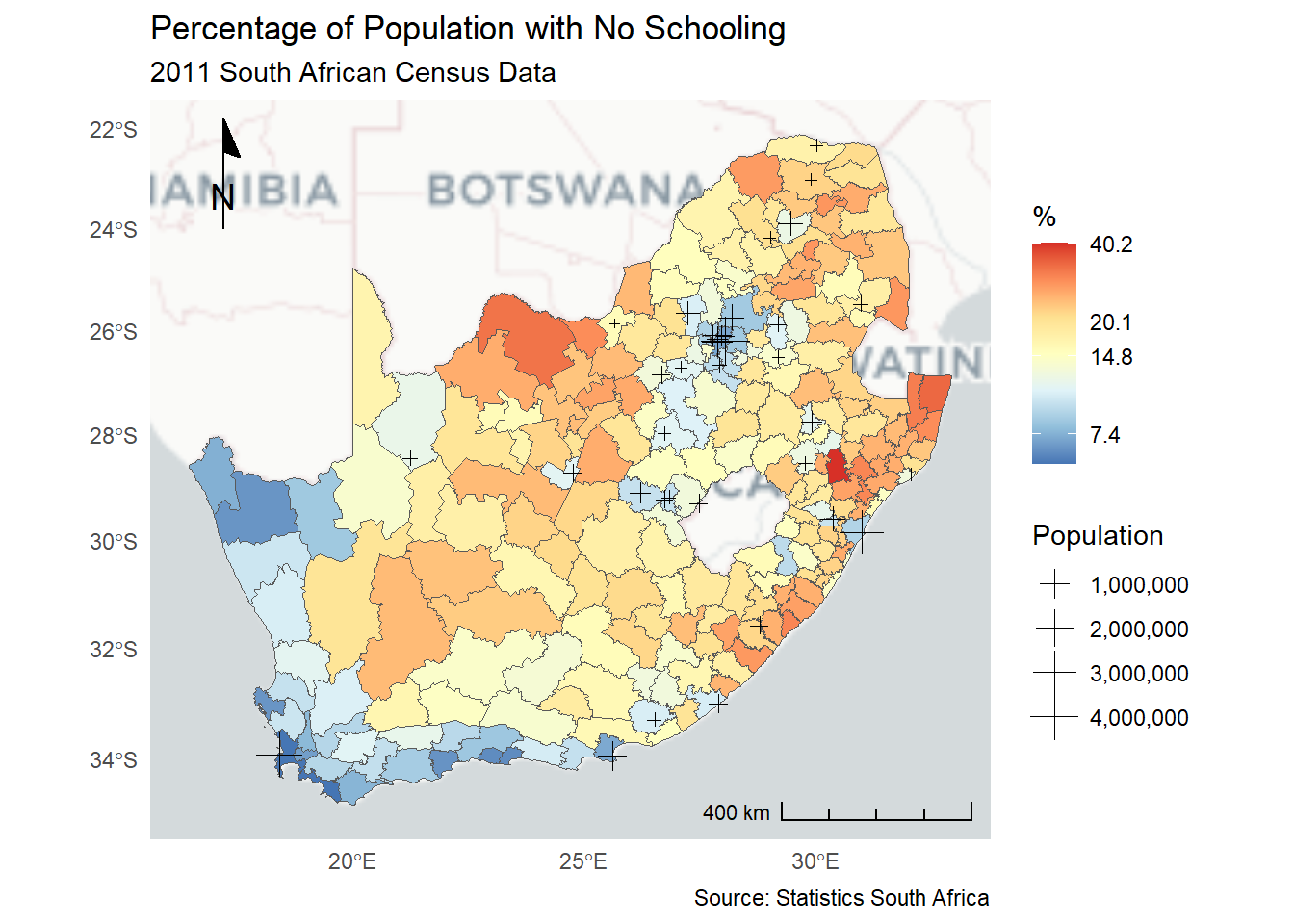
A north arrow and a scale bar can also be added, although including the scale bar generates a warning because the map-to-true-life distance ratio is not actually constant across the map but varies with longitude and latitude (so maybe we should not be adding a scale bar at all?). The argument, location = "tl" is short for top left; location = "br" for bottom right. See ?annotation_north_arrow and ?annotation_scale for further details and options. Note also the use of the last_plot() function to more easily add content to the last ggplot.
In the next example, the locations of South African cities are added to the map, with a symbol drawn in proportion to their population size. The source of the data is a shapefile from https://data.humdata.org/dataset/hotosm_zaf_populated_places. The symbol shape that is specified by pch = 3 has the same numeric coding as those in ?graphics::points (i.e. 0 is a square, 1, is a circle, 2 is a triangle, and so forth).
The function scales::label_comma() forces decimal display of numbers to avoid displaying scientific notation.
The notation [pagkage_name]::[function] is a way of saying in which library/package a specific function is found – the label_comma() function is in the scales library. Sometimes this can be useful to run a function from a package/library without first requiring (loading) it. It can also be useful to avoid the problem when two packages contain a function with the same name. For example, there is a select() function in both the ’raster and dplyr libraries. If you require (load) both of these libraries then the select function in whichever is loaded second will mask the select function in the one loaded first, potentially causing errors or confusions. A way around the problem is to use the :: notation to be specific about which package’s select you wish to use, i.e. raster::select() or dplyr::select().
Slightly confusingly, a shapefile actually consists of at least three files, one with the extension .shp (the coordinate/shape data), one .shx (an index file) and one .dbf (the attribute data). If you use a shapefile you need to make sure you download all of them and keep them together in the same folder.
Labelling using ggsflabel
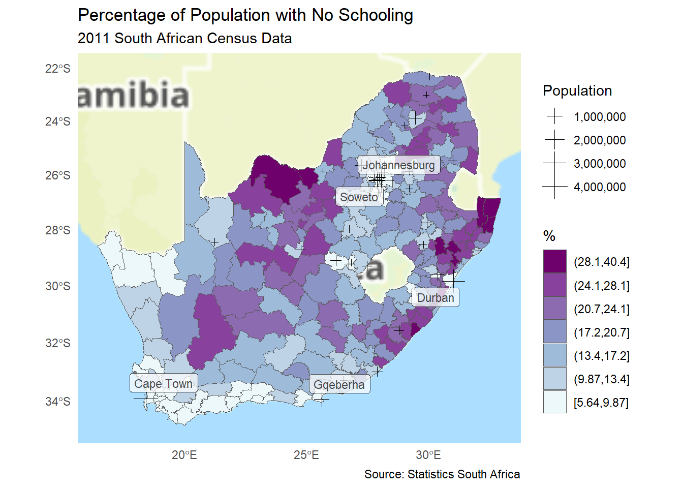
Nice labelling of the cities is provided by ggsflabel, in this example using a pipe |> to filter and only label cities with over a million population. The function geom_sf_label_repel() is designed to stop labels from being placed over each other. We could use last_plot() again but, instead, here is the code in full, going back to using the grouped data, rather than the continuous, log scale, and a different colour palette (just for a bit of variety)
Code
if(!("remotes"%in% installed)) install.packages("remotes", dependencies =TRUE)if(!("ggsflabel"%in% installed)) remotes::install_github("yutannihilation/ggsflabel")require(ggsflabel)ggplot() +annotation_map_tile(type ="thunderforestoutdoors", progress ="none") +geom_sf(data = municipal, aes(fill = No_schooling_gp)) +scale_fill_brewer("%", palette ="BuPu") +geom_sf(data = cities, aes(size = population), pch =3) +scale_size("Population", labels = scales::label_comma()) +geom_sf_label_repel(data = cities |>filter(population >1e6),aes(label = name), alpha =0.7, size =3) +theme_minimal() +# The line below removes some annoying axis titles that otherwise appeartheme(axis.title.x =element_blank(), axis.title.y =element_blank()) +guides(fill =guide_legend(reverse =TRUE)) +labs(title ="Percentage of Population with No Schooling",subtitle ="2011 South African Census Data",caption ="Source: Statistics South Africa" )
Saving the map as a graphic file
Having created the map, it can now be saved as a graphic. If you are not using an R Project to save your files into, you may wish to change your working directory before saving the graphic, using setwd(dir) and substituting dir with the pathname to the preferred directory, or by using Session -> Set Working Directory -> Choose Directory from the dropdown menus. Once you have done so, the last_plot() is easily saved using the function ggsave(). For example, in .pdf format, to a print quality,
Code
ggsave("no_schooling.pdf", device ="pdf", width =6, units ="in",dpi ="print")
Alternatively, we can write directly to a graphics device, using one of the functions bmp(), jpeg(), png(), tiff() or pdf(). For instance,
Code
jpeg("no_schooling.jpg", res =150)last_plot()dev.off()
Creating an interactive map using ggiraph
So far all the maps we have created have been static. This is obviously better for anything that will be printed but, for a website or similar, we may wish to include more ‘interaction’. The package ggiraph package creates dynamic ggplot2 graphs and we can use it to create an interactive map where information about the areas appears as we brush over those areas on the map with the mouse pointer. This is achieved by replacing, in the code, geom_sf() with the geom_sf_interactive() function from ggiraph, specifying the text to show with the tooltip (the example below pastes a number of character elements together without a space between them, hence paste0() but does include a carriage return, \n) and rendering the resulting ggplot2 object with girafe().
Code
if(!("ggiraph"%in% installed)) install.packages("ggiraph", dependencies =TRUE)require(ggiraph)g <-ggplot() +annotation_map_tile(type ="thunderforestoutdoors", progress ="none") +geom_sf_interactive(data = municipal,aes(tooltip =paste0(LocalMunicipalityName.x, "\n",round(No_schooling,1), "%"),fill = No_schooling_gp)) +scale_fill_brewer("%", palette ="BuPu") +theme_minimal() +guides(fill =guide_legend(reverse =TRUE)) +labs(title ="Percentage of Population with No Schooling",subtitle ="2011 South African Census Data",caption ="Source: Statistics South Africa" ) +annotation_north_arrow(location ="tl",style =north_arrow_minimal(text_size =14)) +annotation_scale(location ="br", style ="ticks")girafe(ggobj = g)
Save your workspace
This is the end of Part 1 and is a good place to stop or, at least, take a break. If you won’t be continuing immediately to Part 2 then don’t forget to save your workspace. For example, by using,
Code
save.image("making_maps.RData")
Source Code
---title: "Thematic maps in R (Part 1)"execute: warning: false message: false---```{r}#| include: falseinstalled <-installed.packages()[,1]required <-c("tidyverse", "sf", "RColorBrewer", "gridExtra", "classInt", "ggplot2","ggspatial", "scales", "remotes", "ggiraph", "tmap", "gifski", "mapview")install <- required[!(required %in% installed)]if(length(install)) install.packages(install, dependencies =TRUE, repos ="https://cloud.r-project.org")```## IntroductionThere are lots of ways to produce maps in R. But, however, they are drawn, two things are usually needed to produce a choropleth map of the sort seen in previous sessions:- first, some data;- second, a map to join the data to.The join is usually made possible by the data and the map containing the same variable; for example, by using the same ID codes for all the places in the data as are in the map. This implies that what is contained in the data set are measurements of the places shown in the map. Sometimes maps will come pre-bundled with the data of interest so, in effect, the join has already been made.Once we have the data ready to map (sometimes by 'cleaning' the data before linking them to the map) then R offers plenty of options to produce quick or publication quality maps, which may have either static or dynamic content. The two packages we shall focus on are:- [ggplot2](https://ggplot2-book.org/maps.html){target="_blank"} (mainly in Part 1) and- [tmap](https://cran.r-project.org/web/packages/tmap/vignettes/tmap-getstarted.html){target="_blank"} (mainly in Part 2).However, there are others. Another package we shall be using in this session is [sf](https://cran.r-project.org/web/packages/sf/index.html){target="_blank"}, which provides "support for simple features, a standardized way to encode spatial vector data." What we are mapping in this exercise are vector data -- data for which the geography is ultimately defined by a series of points (two points define a line, a series of lines define a boundary, a boundary demarcates an area, and so forth). The other common geographic representation used in Geographic Information Systems is raster, which is a grid representation of a study region, with each cell in the grid given one or more values to represent what is found there. For raster data, the [stars](https://cran.r-project.org/web/packages/stars/index.html){target="_blank"} and [raster](https://cran.r-project.org/web/packages/raster/index.html){target="_blank"} packages are useful.## Part 1## Getting StartedAs in previous sessions, if you are keeping all the files and outputs from these exercises together in an R Project (which is a good idea) then open that Project now.### Load the dataLet's begin with the easy bit and load the data, which are from [http://superweb.statssa.gov.za](https://superweb.statssa.gov.za/webapi/jsf/login.xhtml){target="_blank"}. These includes the variable `No_schooling` which is the percentage of the population without schooling per South African municipality in 2011.```{r}# A quick check to see if the Tidyverse packages are installed...installed <-installed.packages()[,1]if(!("tidyverse"%in% installed)) install.packages("tidyverse",dependencies =TRUE)require(tidyverse)# Read-in the data directly from a web location. The data are in .csv formateducation <-read_csv("https://github.com/profrichharris/profrichharris.github.io/raw/main/MandM/data/education.csv")# Quick check of the data by looking at the top three rowsslice_head(education, n =3)```### Loading the mapWe have the data but now we need a 'blank map' of the same South African municipalities to map it. It is read-in below in [geoJSON](https://en.wikipedia.org/wiki/GeoJSON){target="_blank"} format but it would not have been unusual if it had been in .shp (shapefile) or .kml format, instead. The source of the data is [https://dataportal-mdb-sa.opendata.arcgis.com/](https://dataportal-mdb-sa.opendata.arcgis.com/datasets/439676d2f2f146889a6eb92da80db780_0/about){target="_blank"}. There are several ways of reading this file into R but it is better to use the `sf` package because older options such as `maptools::readShapePoly()` (which was for reading shapefiles) or `rgdal::readOGR` are either deprecated already or in the process of being retired.```{r}# Another quick check to make sure that various libraries have been installedif(!("proxy"%in% installed)) install.packages("proxy")if(!("sf"%in% installed)) install.packages("sf", dependencies =TRUE)require(sf)# Use the read_sf() function from the sf library to read in a digital map of the study areamunicipal <-read_sf("https://github.com/profrichharris/profrichharris.github.io/raw/main/MandM/boundary%20files/MDB_Local_Municipal_Boundary_2011.geojson")```</br>If we now look at the top of the `municipal` object then we find it is of class `sf`, which is short for [simple features](https://r-spatial.github.io/sf/articles/sf1.html){target="_blank"}. It has a vector geometry (it is of type multipolygon) and has its coordinate reference system (CRS) set as [WGS 84](https://gisgeography.com/wgs84-world-geodetic-system/){target="_blank"}. It also contains some attribute data, although not the schooling data we are looking to map.```{r}slice_head(municipal, n =1)```Here are just the attribute data```{r}st_drop_geometry(municipal) |>slice_head(n =5)```And here is the 'blank' map, drawn using `plot{sf}`, which is the 'base' way of plotting `sf` objects.```{r}par(mai=c(0, 0, 0, 0)) # Removes the plot marginsmunicipal |>st_geometry() |>plot()```Had it been necessary to set the coordinate reference system (CRS) then the function `st_set_crs()` would be used. Instead, and just for fun, we will change the existing CRS: here is the map transformed on to a 'south up' coordinate reference system, achieved by changing its [EPSG code](https://epsg.io/){target="_blank"} to 2050 with the function `st_transform()`. I have no idea why you would want to do this or what the projection is actually used for but, more generally, the `st_transform` is useful for, say (not here, but in other cases), converting between the UK National Grid system (EPSG:27700) and longitude and latitude (EPSG:4326), or making sure the maps you are working with are all using the same CRS, which would be necessary for various GIS ([Geographic Information Systems](https://www.ordnancesurvey.co.uk/gis){target="_blank"}) type operations.```{r}par(mai=c(0, 0, 0, 0))municipal |>st_transform(2050) |>st_geometry() |>plot()```{width=75}<font size = 3>Note how functions with the `sf` library tend to start with `st_`. Personally, I find this slightly confusing and I am not sure it makes it easier to find what I looking for in the package's help pages but it is consistent for the functions and methods that operate on spatial data and is, I believe, short for spatial type.</font>### sf and spAt the risk of over-simplification, `sf` (simple features) can be viewed as a successor to the earlier `sp` (spatial) and related packages, which are well documented in the book [Applied Spatial Data Analysis with R](https://link.springer.com/book/10.1007/978-1-4614-7618-4){target="_blank"}. Sometimes other packages are still reliant on `sp` and so the spatial objects need to be changed into sp's native format prior to use. ```{r}# From sf to spmunicipal_sp <-as(municipal, "Spatial")class(municipal_sp)# From sp to sfmunicipal_sf <-st_as_sf(municipal_sp)class(municipal_sf)```The need for this ought to be less frequent now that `sf` is well established and `sp` deprecated.## Joining the attribute data to the mapIf we look again at the map and schooling data, we find that they have two variables in common which suggests a means to join them together based on a common variable.```{r}# The variables that they appear to have in common...intersect(names(municipal), names(education))```This is encouraging but, in this example, we need to be careful using the municipal names because not all of those in the map are in the education data or vice versa. Although the variable `LocalMunicipalityName` is present in both the map and education data, the variable is not actually the same in both because of different ways of spelling the names of places. The following code shows where one is not the same as the other.```{r}# anti_join() returns all rows from x without a match in yanti_join(municipal, education, by ="LocalMunicipalityName")anti_join(education, municipal, by ="LocalMunicipalityName")```Fortunately, the municipal codes are consistent even where the names are not, which is why place codes and IDs are generally better than using names when joining data. Names are often subject to sometimes subtle variations that can upset the intended join. ```{r}# The municipality codes are consistent in the map and data; there are none that do not match.anti_join(municipal, education, by ="LocalMunicipalityCode")anti_join(education, municipal, by ="LocalMunicipalityCode")```We therefore join the data to the map using the variable `LocalMunicipalityCode` and check that the schooling data are now attached to the map.```{r}municipal <-left_join(municipal, education, by ="LocalMunicipalityCode")names(municipal)```{width=75}<font size = 3>Note that the variables `LocalMunicipalityName.x` and `LocalMunicipalityName.y` have been created in the process of the join. This is because although we did not use `LocalMunicipalityName` for the join, that variable name is present in both the map and the data and is therefore duplicated when they are joined together -- `municipal$LocalMunicipalityName` becomes `municipal$LocalMunicipalityName.x` and `education$LocalMunicipalityName` creates `municipal$LocalMunicipalityName.y`.</font>## Mapping the data### Using `plot{sf}`The 'one line' way of plotting the data is to use the in-built `plot()` function for `sf`.```{r}plot(municipal["No_schooling"])```As a 'rough and ready' way to check for spatial variation and patterns in the data, it is quick and easy. It is important to specify the variable(s) you wish to include in the plot -- `plot(municipal["No_schooling"])` in the example above -- or else it will try and plot all of them in the map's data, up to the value specified by the argument `max.plot`, which has a default of nine.```{r}plot(municipal)```</br>The map can be customised. For example,```{r}if(!("RColorBrewer"%in% installed)) install.packages("RColorBrewer",dependencies =TRUE)require(RColorBrewer)plot(municipal["No_schooling"], key.pos =1, breaks ="jenks", nbreaks =7,pal =rev(brewer.pal(7, "RdYlBu")),graticule =TRUE, axes =TRUE,main ="Percentage of Population with No Schooling")```Have a read through the documentation at `?sf::plot` to get a sense of what the various arguments do. Try changing them and see if you can produce a map with six equal interval breaks, for example.Note the use of the [RColorBrewer package](https://cran.r-project.org/web/packages/RColorBrewer/index.html){target="_blank"} and its `brewer.pal()` function. `RColorBrewer` provides colour palettes based on [https://colorbrewer2.org/](https://colorbrewer2.org/){target="_blank"} and has been used to create a diverging red-yellow-blue colour palette that is reversed using the function `rev()` so that red is assigned to the highest values, not lowest. A 'natural breaks' (jenks) classification with 7 colours has been used (`breaks = "jenks", nbreaks = 7`).### Thinking about the map classesIt is obvious, but under-appreciated, that what we see in a map in a function of how the map is constructed, including the map classes used. Here is the same underlying map but with equal interval breaks instead:```{r}plot(municipal["No_schooling"], key.pos =1, breaks ="equal", nbreaks =7,pal =rev(brewer.pal(7, "RdYlBu")),graticule =TRUE, axes =TRUE,main ="Percentage of Population with No Schooling")```... and here it is with quantile breaks:```{r}plot(municipal["No_schooling"], key.pos =1, breaks ="quantile", nbreaks =7,pal =rev(brewer.pal(7, "RdYlBu")),graticule =TRUE, axes =TRUE,main ="% of Population with No Schooling")```Clearly the maps above do not appear exactly the same. The geographical patterns and therefore the geographical information that we view in the map change with the number, colouring and widths (ranges) of the map classes. Ideally, these should be set to reflect the distribution of the data and what is being look for in it.Let's explore that distribution for a moment and how the various map classes used above end up dividing it up. The following histograms show the break points in the distributions used in the various maps. The code works by creating a list of plots (specifically, a list of ggplots, see below) -- one plot each for the jenks, equal and quantile styles -- and then, using a package called [gridExtra](https://cran.r-project.org/web/packages/gridExtra/index.html){target="_blank"}, to arrange those plots into a single grid. However, the code matters less than what it reveals, which is that [Jenks](http://wiki.gis.com/wiki/index.php/Jenks_Natural_Breaks_Classification){target="_blank"} or other 'natural breaks' classifications are reasonably good for identifying break points that reflect the distribution of the data in the absence of the user having cause to set those break points in some other way.I am not suggesting you need to follow these exact steps every time you want to map but some data. BUT thinking about the distribution of the data is always important to avoid creating maps that give the wrong impression of the prevalence or otherwise of values in the data. For example, if you use a [quantile classification](https://gisgeography.com/quantile-classification-gis/){target="_blank"} with, say, 4 breaks, it will create four map classes, each containing approximately one quarter of the data, even if some of the values in those classes are rarely found and are unusual when compared to others in the same class. An [equal interval classification](https://gisgeography.com/equal-interval-classification-gis/){target="_blank"} will not have this problem.```{r, message=FALSE, warning=FALSE, fig.height=6}if(!("gridExtra" %in% installed)) install.packages("gridExtra", dependencies = TRUE)if(!("classInt" %in% installed)) install.packages("classInt", dependencies = TRUE)require(gridExtra)require(classInt)styles <- c("jenks", "equal", "quantile")g <- lapply(styles, \(x) { ggplot(municipal, aes(x = No_schooling)) + geom_histogram(fill = "light grey") + xlab("% of Population with No Schooling") + geom_vline(xintercept = classIntervals(municipal$No_schooling, n = 7, style = x)$brks, col = "dark red") + geom_rug() + theme_minimal() + ggtitle(paste(x,"classification")) })# The step below brings together, in a grid, the list of three different plots# created abovegrid.arrange(grobs = g)```</br>For further information on using `plot{sf}` see [here](https://r-spatial.github.io/sf/articles/sf5.html){target="_blank"} and look at the help menu, `?sf::plot`.## Using `ggplot2`Whilst the `plot()` function for `sf` objects is useful for producing quick maps, I prefer [ggplot2](https://ggplot2.tidyverse.org/){target="blank"} for better quality ones that I am wanting to customise or annotate in particular ways, or to include in a research publication or report. We already have seen examples of `ggplot2` output in earlier sessions and also in the histograms above.ggplot2 is based on [The Grammar of Graphics](https://link.springer.com/book/10.1007/0-387-28695-0){target="_blank"}. It's a simplification of the 'grammar' but I find it easiest to think of it, initially, in four stages:1. Say which data are to be plotted;2. Say which aesthetics of the chart (e.g. colour, line type, point size) will vary with the data (or just be constant);3. Say which types of plots (which 'geoms') are to feature in the chart;4. (Optional customisation) change other attributes of the chart to add titles, rename the axis labels, and so forth.As an example, and in the code chunk below, those four stages are applied to a boxplot showing the distribution of the no schooling variable by South African Provinces.First, the `data = municipal`.Second, consulting with [the ggplot2 cheatsheet](https://www.rstudio.com/resources/cheatsheets/){target="_blank"}, I find that the aesthetics, `aes()`, for the boxplot, require a discrete `x` and a continuous `y`, which are provided by `ProvinceName` and `No_schooling`, respectively. `ProvinceName` has also been used to assign a `fill` colour to each box.Third, the optional changes arise from me preferring `theme_minimal()` to the default style, although I have then modified it to remove the legend, change the angle of the text on the x-axis, remove the x-axis label and change the y-axis label. I did not have to do any of this; I just preferred it.```{r}require(ggplot2)ggplot(data = municipal, aes(x = ProvinceName, y = No_schooling,fill = ProvinceName)) +geom_boxplot() +theme_minimal() +theme(legend.position ="none", axis.text.x =element_text(angle =45)) +xlab(element_blank()) +ylab("% No schooling within municipalities")```</br>Let's now take that same general process and apply it to create a map, using the same `RColorBrewer` colour palette as previously and adding the map using `geom_sf` (for a full list of geoms available for ggplot2 see [here](https://ggplot2.tidyverse.org/reference/){target="_blank"}). The line `scale_fill_distiller` is an easy way to shade the map using the colour palette from `RColorBrewer` and`labs()` adds labelling. The steps are the same: specify the data; specify the aesthetics; specify the geom (now of type `sf`, because it is a spatial feature); add the customisation.```{r}ggplot(municipal, aes(fill = No_schooling)) +geom_sf() +scale_fill_distiller("%", palette ="RdYlBu") +theme_minimal() +labs(title ="Percentage of Population with No Schooling",subtitle ="2011 South African Census Data",caption ="Source: Statistics South Africa" ) ```</br>Presently the map has a continuous shading scheme -- you can see it in the map's legend. This can be changed to discrete map classes and colours by converting the continuous `municipal$No_schooling` variable to a factor, using the `cut()` function, here with break points found using `ClassIntervals(style = "jenks")`. Because we have then changed from continuous to discrete (categorised) data but still want to use an `RColorBrewer` palette, so `scale_fill_brewer()` replaces `scale_fill_distiller()`, wherein the argument `direction = -1` reverses the `RdYlBu` palette so that the highest values are coloured red. Adding `guides(fill = guide_legend(reverse = TRUE))` reverses the legend so that the highest values are on top in the legend, which is another preference of mine. It just seems kind of logical to me to have the highest values highest in the legend.```{r}# Find the break points in the distribution using a Jenks classificationbrks <-classIntervals(municipal$No_schooling, n =7, style ="jenks")$brks# Factor the No_schooling variable using those break pointsmunicipal$No_schooling_gp <-cut(municipal$No_schooling, brks,include.lowest =TRUE)ggplot(municipal, aes(fill = No_schooling_gp)) +geom_sf() +scale_fill_brewer("%", palette ="RdYlBu", direction =-1) +theme_minimal() +guides(fill =guide_legend(reverse =TRUE)) +labs(title ="Percentage of Population with No Schooling",subtitle ="2011 South African Census Data",caption ="Source: Statistics South Africa" ) ```At this point, we may note that the four stages of the map production that I referred to earlier was an over-simplification and we can add a fifth (but it is the fourth below; sorry to be confusing):1. Say which data are to be plotted;2. Say which aesthetics of the chart (e.g. colour, line type, point size) will vary with the data;3. Say which types of plots (which 'geoms') are to feature in the chart -- geom_sf for mapping;4. (the new one) 'Scale' the data -- in the above examples, link the mapped variables to map classes and colour codes. The scaling is what `scale_fill_...` was doing;5. (Optional customisation) change other attributes of the chart to add titles, rename the axis labels, and so forth.We could also use the scaling to more literally scale (or transform) the data, in a mathematical sense, by using a log scale to plot the data. This will require the original data, before we converted it to factors:```{r}ggplot(municipal, aes(fill = No_schooling)) +geom_sf() +scale_fill_distiller("%", palette ="RdYlBu", trans ="log") +theme_minimal() +labs(title ="Percentage of Population with No Schooling",subtitle ="2011 South African Census Data",caption ="Source: Statistics South Africa" ) ```The legend of that map would look nicer with the values formatted to a more sensible number of decimal places:```{r}ggplot(municipal, aes(fill = No_schooling)) +geom_sf() +scale_fill_distiller("%", palette ="RdYlBu", trans ="log", label = \(x) sprintf("%.1f", x)) +theme_minimal() +labs(title ="Percentage of Population with No Schooling",subtitle ="2011 South African Census Data",caption ="Source: Statistics South Africa" ) ```### Annotating the map with `ggspatial`Having created the basic map using `ggplot2`, we can add some additional map elements using [ggspatial](https://cran.r-project.org/web/packages/ggspatial/index.html){target="_blank"} -- a package that provides some extra cartographic functions. The following code chunk adds a backdrop to the map. Different backgrounds (alternative map tiles) can be chosen from the list at `rosm::osm.types()`; see [here](http://leaflet-extras.github.io/leaflet-providers/preview/index.html){target="_blank"} for what they look like.Before running the code, we may note a change from the previous code chunk (above) which is in addition to installing and requiring `ggspatial` and adding the map tile as a backdrop. Specifically, if you look at the previous code chunk you will find that the data, `municipal` are handed to ggplot in the top line, `ggplot(municipal, ...)`, where the first argument is the data one. In other words, `ggplot(municipal, ...)` is the same as, `ggplot(data = municipal, ...)` (check the help file, `?ggplot2::ggplot` to confirm this). By specifying the data in the top line, in essence this sets `data = municipal` as a global parameter for the plot: it is where ggplot will, by default, now look for the variable called for in `aes(fill = No_schooling_gp)` and where it will look for other variables too. Whilst this would work just fine in the code immediately below, a little later I introduce a second `geom_sf` into the plot and no longer want `municipal` to be the default choice for all the aesthetics of the chart, just some of them. To pre-empt any problems that might otherwise arise, I no longer specify `municipal` as the default dataset in my `ggplot()` but, instead, specifically name `municipal` where I want to use it, which is as the `fill` data, in the line `geom_sf(data = municipal, aes(fill = No_schooling_gp))`. This will leave me free to associate other data with different aesthetics in due course. More simply, if you set the `data =` argument and also any aesthetics, `mapping = aes()` in the `ggplot(...)` line of the code, then you are basically saying "use these for everything that follows" unless you override them by saying what you want for each specific geom.```{r}if(!("ggspatial"%in% installed)) install.packages("ggspatial",dependencies =TRUE)require(ggspatial)ggplot() +annotation_map_tile(type ="cartolight", progress ="none") +geom_sf(data = municipal, aes(fill = No_schooling_gp)) +scale_fill_brewer("%", palette ="RdYlBu", direction =-1) +theme_minimal() +guides(fill =guide_legend(reverse =TRUE)) +labs(title ="Percentage of Population with No Schooling",subtitle ="2011 South African Census Data",caption ="Source: Statistics South Africa" ) ```<br>Or, using our previous log scale,```{r}ggplot() +annotation_map_tile(type ="cartolight", progress ="none") +geom_sf(data = municipal, aes(fill = No_schooling)) +scale_fill_distiller("%", palette ="RdYlBu", trans ="log", label = \(x) sprintf("%.1f", x)) +theme_minimal() +labs(title ="Percentage of Population with No Schooling",subtitle ="2011 South African Census Data",caption ="Source: Statistics South Africa" ) ```</br>A north arrow and a scale bar can also be added, although including the scale bar generates a warning because the map-to-true-life distance ratio is not actually constant across the map but varies with longitude and latitude (so maybe we should not be adding a scale bar at all?). The argument, `location = "tl"` is short for top left; `location = "br"` for bottom right. See `?annotation_north_arrow` and `?annotation_scale` for further details and options. Note also the use of the `last_plot()` function to more easily add content to the last ggplot.```{r}last_plot() +annotation_north_arrow(location ="tl",style =north_arrow_minimal(text_size =14)) +annotation_scale(location ="br", style ="ticks")```### Adding point symbols to the mapIn the next example, the locations of South African cities are added to the map, with a symbol drawn in proportion to their population size. The source of the data is a [shapefile](https://desktop.arcgis.com/en/arcmap/latest/manage-data/shapefiles/what-is-a-shapefile.htm){target="_blank"} from [https://data.humdata.org/dataset/hotosm_zaf_populated_places](https://data.humdata.org/dataset/hotosm_zaf_populated_places){target="_blank"}. The symbol shape that is specified by `pch = 3` has the same numeric coding as those in `?graphics::points` (i.e. 0 is a square, 1, is a circle, 2 is a triangle, and so forth).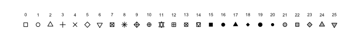The function `scales::label_comma()` forces decimal display of numbers to avoid displaying scientific notation. {width=75}<font size = 3>The notation `[pagkage_name]::[function]` is a way of saying in which library/package a specific function is found -- the `label_comma()` function is in the `scales` library. Sometimes this can be useful to run a function from a package/library without first requiring (loading) it. It can also be useful to avoid the problem when two packages contain a function with the same name. For example, there is a `select()` function in both the '`raster` and `dplyr` libraries. If you require (load) both of these libraries then the select function in whichever is loaded second will mask the select function in the one loaded first, potentially causing errors or confusions. A way around the problem is to use the `::` notation to be specific about which package's select you wish to use, i.e. `raster::select()` or `dplyr::select()`.</font>```{r}if(!("scales"%in% installed)) install.packages("scales", dependencies =TRUE)download.file("https://github.com/profrichharris/profrichharris.github.io/blob/main/MandM/boundary%20files/hotosm_zaf_populated_places_points_shp.zip?raw=true","cities.zip", mode ="wb", quiet =TRUE)unzip("cities.zip")read_sf("hotosm_zaf_populated_places_points.shp") |>filter(place =="city") |>mutate(population =as.numeric(population)) -> citieslast_plot() +geom_sf(data = cities, aes(size = population), pch =3) +scale_size("Population", labels = scales::label_comma())```{width=75}<font size = 3>Slightly confusingly, a shapefile actually consists [of at least three files](https://www.esri.com/content/dam/esrisites/sitecore-archive/Files/Pdfs/library/whitepapers/pdfs/shapefile.pdf){target="_blank"}, one with the extension .shp (the coordinate/shape data), one .shx (an index file) and one .dbf (the attribute data). If you use a shapefile you need to make sure you download all of them and keep them together in the same folder.</font>### Labelling using `ggsflabel`Nice labelling of the cities is provided by [ggsflabel](https://github.com/yutannihilation/ggsflabel){target="_blank"}, in this example using a pipe `|>` to filter and only label cities with over a million population. The function `geom_sf_label_repel()` is designed to stop labels from being placed over each other. We could use `last_plot()` again but, instead, here is the code in full, going back to using the grouped data, rather than the continuous, log scale, and a different colour palette (just for a bit of variety)```{r}if(!("remotes"%in% installed)) install.packages("remotes", dependencies =TRUE)if(!("ggsflabel"%in% installed)) remotes::install_github("yutannihilation/ggsflabel")require(ggsflabel)ggplot() +annotation_map_tile(type ="thunderforestoutdoors", progress ="none") +geom_sf(data = municipal, aes(fill = No_schooling_gp)) +scale_fill_brewer("%", palette ="BuPu") +geom_sf(data = cities, aes(size = population), pch =3) +scale_size("Population", labels = scales::label_comma()) +geom_sf_label_repel(data = cities |>filter(population >1e6),aes(label = name), alpha =0.7, size =3) +theme_minimal() +# The line below removes some annoying axis titles that otherwise appeartheme(axis.title.x =element_blank(), axis.title.y =element_blank()) +guides(fill =guide_legend(reverse =TRUE)) +labs(title ="Percentage of Population with No Schooling",subtitle ="2011 South African Census Data",caption ="Source: Statistics South Africa" ) ```### Saving the map as a graphic fileHaving created the map, it can now be saved as a graphic. If you are not using an R Project to save your files into, you may wish to change your working directory before saving the graphic, using `setwd(dir)` and substituting `dir` with the pathname to the preferred directory, or by using Session -> Set Working Directory -> Choose Directory from the dropdown menus. Once you have done so, the `last_plot()` is easily saved using the function `ggsave()`. For example, in .pdf format, to a print quality,```{r}#| eval: falseggsave("no_schooling.pdf", device ="pdf", width =6, units ="in",dpi ="print")```Alternatively, we can write directly to a graphics device, using one of the functions `bmp()`, `jpeg()`, `png()`, `tiff()` or `pdf()`. For instance, ```{r}#| eval: falsejpeg("no_schooling.jpg", res =150)last_plot()dev.off()```## Creating an interactive map using `ggiraph`So far all the maps we have created have been static. This is obviously better for anything that will be printed but, for a website or similar, we may wish to include more 'interaction'. The package [ggiraph](https://cran.r-project.org/web/packages/ggiraph/index.html){target="_blank"} package creates dynamic `ggplot2` graphs and we can use it to create an interactive map where information about the areas appears as we brush over those areas on the map with the mouse pointer. This is achieved by replacing, in the code, `geom_sf()` with the `geom_sf_interactive()` function from `ggiraph`, specifying the text to show with the `tooltip` (the example below pastes a number of character elements together without a space between them, hence `paste0()` but does include a carriage return, `\n`) and rendering the resulting ggplot2 object with `girafe()`.```{r}if(!("ggiraph"%in% installed)) install.packages("ggiraph", dependencies =TRUE)require(ggiraph)g <-ggplot() +annotation_map_tile(type ="thunderforestoutdoors", progress ="none") +geom_sf_interactive(data = municipal,aes(tooltip =paste0(LocalMunicipalityName.x, "\n",round(No_schooling,1), "%"),fill = No_schooling_gp)) +scale_fill_brewer("%", palette ="BuPu") +theme_minimal() +guides(fill =guide_legend(reverse =TRUE)) +labs(title ="Percentage of Population with No Schooling",subtitle ="2011 South African Census Data",caption ="Source: Statistics South Africa" ) +annotation_north_arrow(location ="tl",style =north_arrow_minimal(text_size =14)) +annotation_scale(location ="br", style ="ticks")girafe(ggobj = g)```## Save your workspaceThis is the end of Part 1 and is a good place to stop or, at least, take a break. If you won't be continuing immediately to Part 2 then don't forget to save your workspace. For example, by using,```{r}save.image("making_maps.RData")```